



580 California St., Suite 400
San Francisco, CA, 94104
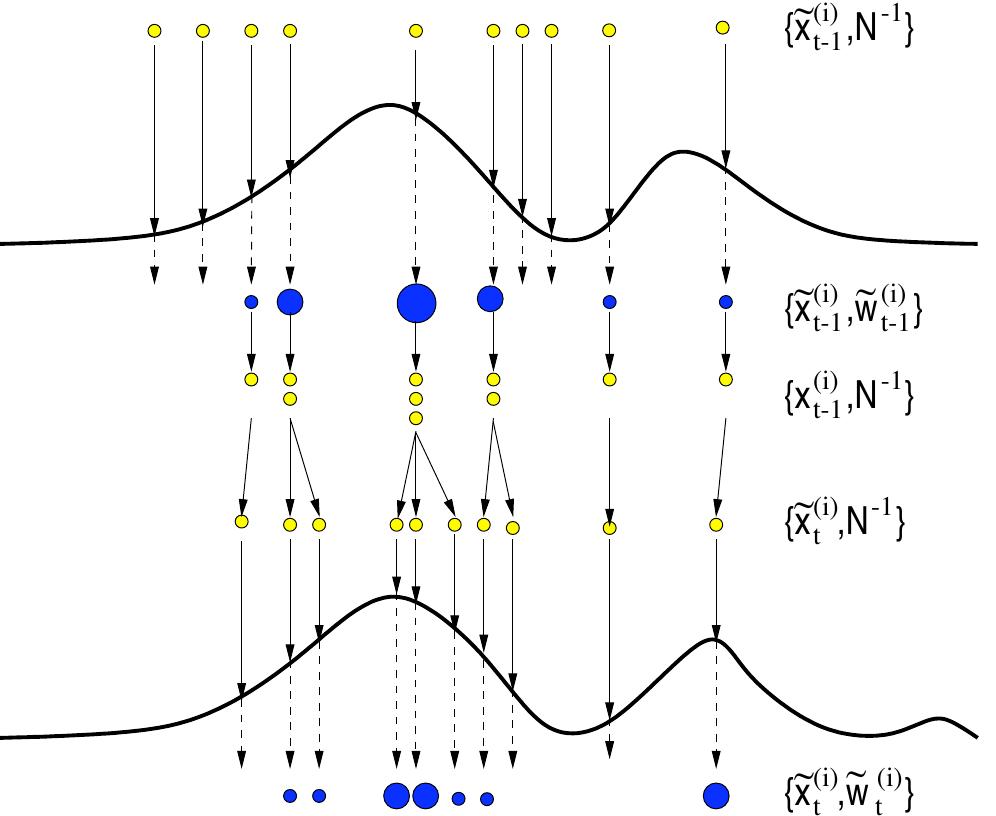
Figure 1: In this example, a particle filter starts at time ¢ — 1 with an unweighted measure (x2, N71}, which provides an approximation of p(xz-1|y1.:-2). For each particle we compute the importance weights using the information at time ¢ — 1. This results in the weighted measure (x, OO, , which yields an approximation p(X:-1|¥1:2-1)- Subsequently, a resampling step selects only the “fittest” particles to obtain the unweighted measure {x,, N-1}, which is still an approximation of p(Xt-1|¥1:t-1) - Finally, the sampling (prediction) step introduces variety, resulting in the measure {x , N-}. where “*$ denotes almost sure convergence and f; : R’= > R’% is some func- tion of interest. For example, it could be the conditional mean, in which case fi (Xo) = Xo, or the conditional covariance of x; with f;(xo%) = xix}; —
Figure source:
