UAV MODELING SIMULATION STABILITY AND CONTROL

*BACHELOR OF ENGINEERING DEGREE/DEGREE WITH HONOURS IN AEROSPACE SYSTEMS ENGINEERING *BEng Final Year Project Report School of Engineering and Technology University of Hertfordshire MODELLING AND SIMULATION OF A UH UAV DYNAMICS Report by LEONINE .F KUNZWA Supervisor DR RASHID ALI Date 27 April 2011 DECLARATION STATEMENT I certify that the work submitted is my own and that any material derived or quoted from the published or unpublished work of other persons has been duly acknowledged (ref. UPR AS/C/6.1, Appendix I, Section 2 – Section on cheating and plagiarism) Student Full Name: LEONINE FUNGAI KUNZWA Student Registration Number: 08177750 Signed: ………………………………………………… Date: SELECT DATE OF SUBMISSION HERE School of Engineering and Technology *BEng Final Year Project Report ABSTRACT Static and dynamic stability was defined and the UAV components contribution to static and dynamic stability was highlighted. The recommended geometric configurations based on desired stability characteristics were outlined. The Longitudinal and lateral derivatives were defined, estimated and analysed. They were estimated using the USF stability and control Datcom (Data Compendium) method. An excel model was used to estimate the motions, calculate the forces, moments and determine the transfer functions for longitudinal and lateral modes. A Simulink model1 was developed to predict the dynamic characteristic of the existing UH UAV (MAK.2). Another Simulink model was developed to overcome the drawbacks of Simulink model1. The Simulink model was interfaced with flight gear and linked to excel model. Modelling and simulation of UH-UAV dynamics i School of Engineering and Technology *BEng Final Year Project Report ACKNOWLEDGEMENTS I thank Dr Rashid Ali for his support, motivation and supervision throughout the year. I thank my family for supporting me and my parents for their inspiration and encouragement. I also thank my housemates and friends Mr A Nyakandi, Mr K Kimani, Dr M Choong, Mr R Krish for providing intellectually stimulating company and constructive criticism. I thank Mr M Sakarombe and Mrs Kalama for their support. Modelling and simulation of UH-UAV dynamics ii School of Engineering and Technology *BEng Final Year Project Report TABLE OF CONTENTS DECLARATION STATEMENT ...................................................................................................... i ABSTRACT ................................................................................................................................... i ACKNOWLEDGEMENTS ............................................................................................................ ii TABLE OF CONTENTS .............................................................................................................. iii Nomenclature ...............................................................................................................................1 1. Introduction ..........................................................................................................................2 1.1 History and future of UAV .............................................................................................2 1.2 Aims and objectives ......................................................................................................3 1.2.1 UAV specifications ................................................................................................3 1.2.2 Axis System ...............................................................................................................4 2. Static stability and Control ...................................................................................................4 2.1 UAV Static stability (Cmo>0) ........................................................................................4 2.2 UAV Dynamic stability .......................................................................................................5 2.2.1 UAV Oscillatory motion ..............................................................................................5 2.3 UAV Longitudinal static stability and control .....................................................................6 2.3.1 Contribution of aircraft components to stability ..........................................................6 UAV Wings contribution .......................................................................................................6 UAV fuselage contribution ...................................................................................................7 UAV engine contribution ......................................................................................................7 UAV tail contribution ............................................................................................................7 UAV Stick free and stick fixed stability .................................................................................8 Desirable geometry configuration ........................................................................................9 2.4 UAV Longitudinal control...................................................................................................9 2.4.1 Aerodynamic balance ................................................................................................9 2.5 UAV Directional stability ..................................................................................................10 2.5.1 UAV components contribution .................................................................................10 2.6 UAV Directional control ...................................................................................................10 2.6.1 UAV Roll stability .....................................................................................................11 UAV Components contribution ..........................................................................................11 2.6.2 UAV Roll control ...........................................................................................................11 2.6.3 UAV coupling motions .............................................................................................11 3 Aerodynamic Modelling ..........................................................................................................12 3.1 UAV Moment of inertia ....................................................................................................12 3.2 Aerodynamic forces and Derivatives ...............................................................................12 3.2.1 Longitudinal derivatives ..........................................................................................13 3.2.2 The Lateral Derivatives .........................................................................................15 4 UAV Longitudinal motions ......................................................................................................17 Modelling and simulation of UH-UAV dynamics iii School of Engineering and Technology *BEng Final Year Project Report 4.1 Derivative influence on longitudinal motion .....................................................................18 5 UAV Lateral motion ................................................................................................................19 6 Models and Simulations .........................................................................................................20 6.1 The UAV generic model 1 ...............................................................................................21 6.2 UAV generic model 2 ......................................................................................................22 6.3 UAV generic model 3 ......................................................................................................23 7 Results ...................................................................................................................................25 7.1 Longitudinal dynamics.....................................................................................................25 7.2 UAV responds to Gust and turbulence ............................................................................27 7.3 Lateral Dynamics ............................................................................................................28 8 The UAV Simulink models ......................................................................................................31 8.1 Simulink Model 1 ..........................................................................................................31 8.2 Simulink model 2 ...........................................................................................................38 8.3 The excel model ..............................................................................................................42 9 Linking Simulink model1 with excel model. .............................................................................43 Summary ....................................................................................................................................45 References .................................................................................................................................47 Bibliography ...............................................................................................................................50 APPENDICES ............................................................................................................................51 Modelling and simulation of UH-UAV dynamics iv School of Engineering and Technology *BEng Final Year Project Report Nomenclature a -Local speed of sound r -Yaw rate AR- wing Aspect ratio S -wing reference area ARt- Tail Aspect ratio Sv- Fin reference area ARv- Vertical Aspect ratio St -Tailplane reference area b -Wing span T2 -Time to double amplitude c -Mean aerodynamic chord (mac) u -Axial velocity CD -Drag coefficient U -Total axial velocity CD0- Zero lift drag coefficient v -Lateral velocity Cl -Rolling moment coefficient V - velocity CL- Lift coefficient Vv -Fin volume ratio CLw- Wing lift coefficient Vh-Tailplane volume ratio CLt -Tail lift coefficient w -Normal velocity CH -Elevator hinge moment coefficient W- Weight Cm -Pitching moment coefficient x -Longitudinal coordinate in axis system Cm0- Pitching moment coefficient about X -Axial force component wing -ac Y -Lateral force component Cmα –Cm Cave slope Z -Normal force component Cn- Yawing moment coefficient Β- Sideslip angle Cx -Axial force coefficient γ- Flight path angle Cy -Lateral force coefficient δ -Control angle Cz- Normal force coefficient ε -Downwash angle at tail plane e- Oswald efficiency factor ε0 -Zero lift downwash angle at tail H -Elevator hinge moment ζ -Rudder angle: Damping ratio Ix -Moment of inertia in roll ζd -Dutch roll damping ratio Iy -Moment of inertia in pitch ζp- Phugoid damping ratio Iz -Moment of inertia in yaw ζs- Short period pitching oscillation Kn- Controls fixed static stability margin damping ratio lv -Distance from cg to fin ac point η -Elevator angle lt -Distance from cg to horizontal tail ac θ- Pitch angle L- Lift Rolling moment λ -Eigenvalue m- Mass Λ -Wing sweep angle M -Mach number ξ -Aileron angle M -Pitching moment ρ -Air density N- Yawing moment φ- Roll angle p -Roll rate ψ Yaw angle q -Pitch rate ω -Undamped natural frequency Q -Dynamic pressure Modelling and Simulation of a UH-UAV dynamics 1 School of Engineering and Technology *BEng Final Year Project Report 1. Introduction 1.1 History and future of UAV Unmanned Aerial vehicle (UAV) is defined as a “powered aerial vehicle that uses aerodynamic forces to provide vehicle lift, can fly autonomously or be piloted remotely, can be expendable or recoverable, and can carry a lethal or nonlethal payload”. [1] The concept of UAV first started during American civil war. Balloons carrying explosives were sent to explode in enemy territories. The Japanese also tried the same concept during World War2. A prototype UAV called Operation Aphrodite was introduced by American defence during World War 2 as an attempt to fly manned aircrafts in an unmanned mode. However, the operation wasn’t successful due to lack of technology to control the unmanned vehicle. [2] The USA military used drones named U-2 and Firebee in 1960s for reconnaissance missions. The firebee was extensively used for reconnaissance and combat during The Vietnam War. It was equipped with UV cameras, communications and electronic intelligence. The increase in technology has resulted in high endurance UAV with full combat capabilities. For example, the Predator has 40hrs endurance and the Global hawk has 24hrs endurance. There has been an increase in commercial applications of UAVs. Some of the industries in which UAVs have gained interest are the agricultural sector where UAVs are beings used to spray insecticides, fertiliser and for crop monitoring in large fields. [3] They are also being used in mineral explorations for aerial surveying to find minerals in otherwise inaccessible areas. Some UAVs are being used for coastline monitoring in marine and mobile relay platforms in telecommunications. Other civilian uses of UAVs include news broadcasting, air and ground traffic control for monitoring busy airports and motorways. According to John Keller, America invested $4.5 billion in 2010 on UAV technology. [4] There is a vast range of UAV designs and specifications and each suited for its intended mission. As highlighted above, the use of UAVs is becoming more popular in both defence and environmental research industries. However, there is still high developmental cost. The UAV testing phase has the highest budget in the development cycle. [5] There is also high risk that the UAV might be unstable or fail when subjected to different parameters. One cannot be absolutely sure whether the UAV meets the specifications without test flights. This project is a solution to the problems outlined. Modelling the UAV dynamics will enable a thorough analysis in the behaviour and stability of the UAV at different conditions. Real time simulations will save time cost and eliminate risk. The project is to use MathWorks package (Matlab and Simulink) to model the six degrees of freedom of the dynamics of a particular UAV; and use the model to accurately simulate any UAV by simply changing the variables. This will be achieved by using the equations of motion. This approach has been adopted by companies such as BAE systems when developing the Eagle 150. BAE SYSTEMS Controls Develops Autopilot for Unmanned Aerial Vehicle Using MathWorks Tools. [6] Modelling and Simulation of a UH-UAV dynamics 2 School of Engineering and Technology *BEng Final Year Project Report 1.2 Aims and objectives Aims: • To successfully test flight a completed UH UAV. • To model the six degrees of freedom of the dynamics of the UH UAV. • To predict the static, dynamic stability and control parameters from the simulation. Objectives: • Contributing actively in the construction and test-flight of the UH UAV. • Completing the UAV simulation before the test flight. • Estimating longitudinal and lateral stability and control derivatives. • Developing a UAV model using Matlab and Simulink. • Applying engineering and mathematical problem solving skills. • Managing time efficiently by effective time planning. 1.2.1 UAV specifications The 2011 UH-UAV will be used in the meteorology industry for data collection in the Antarctic. It will be equipped with some sensors and cameras for data collection and recording. Specifications • Operating temperature of -40⁰C • Endurance of 3hrs • Top speed of 65 knots • Radio link radius more than 40km • Maximum weight of 12kg including engine but excluding fuel and payload • Has a detachable payload bay (Modular) • Can accommodate different payload bays • Autonomous Modelling and Simulation of a UH-UAV dynamics 3 School of Engineering and Technology *BEng Final Year Project Report 1.2.2 Axis System 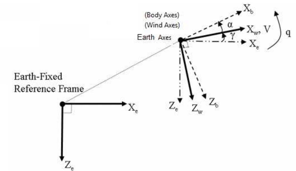Body axis: The axis is fixed on the UAV’s centre of gravity (CG) and moments of inertia are constant. xb axis is along the nose, yb axis is along the wing and zb axis points down. Earth axis: assumes a flat earth and the system is fixed on the surface of the earth. xe,ye,ze axis corresponding to north, east and earth’s centre. [Figure 1.2.2] Wind axis: assumes that the applied forces act on the UAV’s centre of gravity. Figure 1.2.2 axis system (from Matlab help manual by MathWorks 2009) 2. Static stability and Control The UAV’s state of equilibrium is where the sum of forces and moments at its centre of gravity are zero.[7] Stability is the tendency for an aircraft to return to its equilibrium position after a disturbance. The disturbance can be due to various inputs such as turbulence, gusts winds and pilot inputs. The UAV must be stable even after being exposed to these external disturbances. The UAV must be stable in level flight and also manoeuvrable at different speeds to ensure success of the intended mission. The ability for the UAV to easily achieve this with minimal workload is considered as its handling qualities. [8] 2.1 UAV Static stability (Cmo>0) Assuming controls are fixed and displacement is due to atmospheric disturbance. Static stability is the initial tendency for the UAV to return to its equilibrium position after a displacement due to external disturbances. If the UAV return to its equilibrium position after a displacement, then it has positive static stability and if it moves away from its equilibrium position, then it has negative static stability. If the UAV stays at its new position after a displacement, it is considered to have neutral static stability. [9] Positive static stability is stable. Negative static stability is unstable. Neutral static stability is neither stable nor unstable hence neutral. Modelling and Simulation of a UH-UAV dynamics 4 School of Engineering and Technology *BEng Final Year Project Report 2.2 UAV Dynamic stability Assuming controls are fixed and displacement is due to atmospheric disturbance. 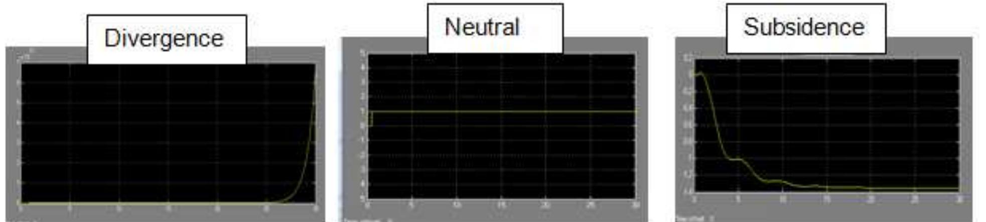Dynamic stability is the motion of the UAV with respect to time after a disturbance from its equilibrium position. If the maximum displacement of the UAV from its equilibrium position decreases with time, then the UAV has positive dynamic stability (Figure 2.2) subsidence motion). However, if it increases with time then it has negative dynamic stability (Figure 2.2) divergence motion). Is the motion remain constant with time; the UAV has neutral dynamic stability.[10] Figure ‎2.2 Dynamic stability 2.2.1 UAV Oscillatory motion The UAV can be statically stable but dynamically unstable. The UAV must be statically stable to be dynamically stable but static stability does not guarantee dynamic stability. If the UAV has positive static stability but negative dynamic stability, it will have divergent oscillation. 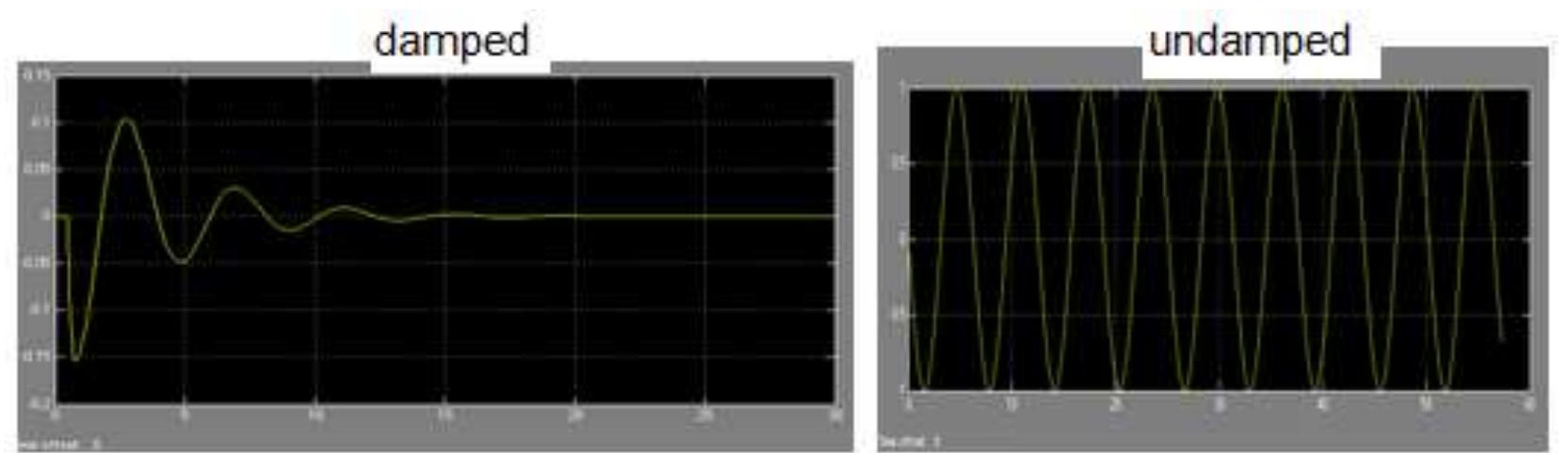If the UAV has positive static stability but neutral dynamic stability, it will have undamped oscillation or simple harmonic motion. The design aim is for the UAV to have both positive and dynamic stability, thus a damped oscillation. If this condition is mate the UAV will always return to its equilibrium position after a disturbance.[11] Figure 2.2.1 Oscillatory motions Modelling and Simulation of a UH-UAV dynamics 5 School of Engineering and Technology *BEng Final Year Project Report 2.3 UAV Longitudinal static stability and control The trim angle of attack is the angle of attack at which the pitching moments are zero.[12] If a UAV with a negative static longitudinal stability is disturbed from its trim angle of attack, it will continue to pitch away from the trim angle of attack or equilibrium position. This characteristic is not desirable. The UAV is said to have neutral static longitudinal stability if when disturbed from its trim position will remain at the new angle of attack. The UAV is said to be longitudinally statically stable if a nose-up change in angle of attack from trim point result in a nose down restoring moment that will return the UAV to its trim angle of attack or equilibrium position . This is a desirable design characteristic as it results in the UAV being trimmed at wide range of desired flight speeds. 2.3.1 Contribution of aircraft components to stability Assuming it is a convectional configuration. UAV Wings contribution Aerodynamic centre (AC) is the point at which the change of moment due to change of angle of attack is zero. It is the point of lift on a wing, Cmα =0. [13] The wing contribution to the stability is determined by the position of the AC with respect to the CG position of the UAV. If the CG is forward of the AC, the aircraft will have a natural nose down pitching tendency that will restore the UAV to its equilibrium position; after an up- gust disturbance. This is considered to be a stable condition, hence it is desirable. If the CG is aft of the AC, an up-gust will cause an increase of lift on the AC that will rotate the UAV about the CG, creating a moment that will rotate the UAV away from the equilibrium position. This is an unstable condition and hence undesirable.[14] Therefore the CG must be forward of the AC when designing the UAV. The aerofoils also contribute to stability. Positive cambered aerofoils cause nose down pitching moment, whereas negative cambered aerofoils produce nose up pitching moment. Therefore a negative cambered aerofoil should be chosen for a forward CG. This will ensure stability in pitch because the natural pitch down tendency will have a nose up counteracting moment due to the negative camber. Coefficient of pitching moment due to wing contribution 2.1 [15] Modelling and Simulation of a UH-UAV dynamics 6 School of Engineering and Technology *BEng Final Year Project Report UAV fuselage contribution In the presence of an up-gust, the fuselage will have a destabilising pitching moment [16] Coefficient of pitching moment due to fuselage [17] 2.2 K2 –k1 is the body fineness ratio correction factor S is wing area c is the wing aerodynamic chord wf is the average fuselage sections αow is wing zero lift angle relative to fuselage if is incidence of the fuselage camber line relative to the fuselage ∆x is fuselage length increment [18] UAV engine contribution If the UAV’s engine axis is at an angle with the free stream; the airflow is turned towards the engine axis creating a side force on the propeller shaft. For a forward mounted propeller engine, at positive angles of attack; the force will cause a nose up pitching moment. This will be destabilising. If the propeller engine is mounted aft of the cg; the upward force will result in a nose-down pitching moment. This is a stabilising moment. [19] The engine contributes to Cmα or Cmά. The engine effects can be obtained from wing tunnel data. Hence the UAV should have an aft mounted engine. UAV tail contribution Assuming a symmetrical aerofoil. This is a stabilising component of the UAV. It should produce both upward and downward force when required. For instance, if there is a disturbance due to upward gust; the UAV will pitch up. An upward force (positive lift) is produced by the tail creating a nose-down restoring moment. When subjected to an upward-gust the UAV will pitch down. The tail will produce a down force (negative lift) creating a nose-up restoring moment. The effectiveness of the tail on stability is determined by its area and the distance from the aft cg to the tail ac. The positioning of the tail above the wing line is significant considering downwash effects.[20] Modelling and Simulation of a UH-UAV dynamics 7 School of Engineering and Technology *BEng Final Year Project Report Coefficient pitching moment due to tail 2.3 [21] Downwash angle 2.4 εo is downwash at zero angle of attack dε/dα is change in downwash with respect to angle of attack [22] 2.5 CLw is wing lift coefficient (from aerofoil data) ARw is wing aspect ratio CLαw is wing lift curve slope Coefficient of pitching moment of the UAV Cmo = Cmot+ Cmof+ Cmow Cmα=Cmαt + Cmαw + Cmαf UAV Stick free and stick fixed stability Stick free is when the controls surfaces are free to move and can be displaced from neutral point when subjected to atmospheric disturbances. This reduces the overall stabilising surface. Stick fixed is when the control surfaces are in a fixed position and they are not free to move when subjected to atmospheric disturbances. This ensures better stability. Hence the UAV will have stick fixed stability.[23] At neutral point, Cmα=0 The following equation is used to determine the neutral point 2.6 Modelling and Simulation of a UH-UAV dynamics 8 School of Engineering and Technology *BEng Final Year Project Report Desirable geometry configuration  CG forward of the AC.  A negative cambered wing aerofoil.  An aerodynamic balanced tail with symmetrical aerofoil.  An aft mounted engine.  Smaller fuselage area.  Stick fixed stability. 2.4 UAV Longitudinal control The pitch is controlled by deflection of elevators. Factors to consider are 1. Hinge moments: These are moments exerted on the control surface The control surface must overcome the hinge moments. This determines the magnitude of torque the servo motors must produce, to move the control surface. Therefore when sizing up the UAV control surfaces, ensure that the servos selected can meet the control force requirements. However cost of servo motors, size and weight must be also be considered. 2. Elevator effectiveness: is the measure of how effective the elevator is at producing the desired pitching moment. [24] 3. Trim: The UAV is trimmed when the forces and moments acting on the UAV are in equilibrium. Cm=0 in trim [25] 2.4.1 Aerodynamic balance Assuming the centre of gravity is at the most forward position. Worst case scenario is when the UAV is landing with flaps and landing gear deployed. The UAV will have a large negative (nose down) pitching moment which has to be counteracted by the elevator. If the UAV CG is forward of the most estimated forward CG; the UAV will have to be trimmed at lower angles of attack. This result in increased landing speeds.[26] The UAV should be designed to have low landing speeds. Modelling and Simulation of a UH-UAV dynamics 9 School of Engineering and Technology *BEng Final Year Project Report 2.5 UAV Directional stability Directional stability is the tendency for the UAV to return to its equilibrium position when subjected to an atmospheric yaw disturbance. Assuming the UAV is trimmed at non sideslip flight. If the UAV return to its equilibrium position (zero sideslip angle) after a yaw displacement, then it has positive directional stability and if it moves away (increasing sideslip angle) from its trimmed sideslip, then it has negative directional stability. If the UAV stays at the same sideslip angle after a yaw displacement, it is considered to have neutral directional stability.[27] , The UAV must be designed for positive directional stability (Cnβ>0) 2.5.1 UAV components contribution Fuselage: for the UAV to be directionally stable, the area of the fuselage aft of the CG must be greater than the fuselage area forward of CG. 2.7 Kn is wing body interference factor Krl is correction factor Sfs is the projected area of fuselage lf is fuselage length Engine: aft engine is directionally stabilizing Vertical tail: directionally stabilising 2.8 Dorsal fin: directionally stabilising with reduced drag Rudder: Fixed rudder increases the vertical area thus increasing directional stability Wing contribution is Cnβw=CL²/4πAR [28] The yawing moment coefficient due to sideslip of the UAV Cnβ= Cnβf + Cnβw+ Cnβv 2.9 2.6 UAV Directional control The rudder provides directional control by producing a yaw moment about the CG. The yaw moment produced is a product of force due to rudder deflection and its distance from the CG. Its effectiveness is the rate of change of yaw moment with respect to rudder deflection angle. [29]. The UAV rudder size must be big enough to allow recovery from spin. Modelling and Simulation of a UH-UAV dynamics 10 School of Engineering and Technology *BEng Final Year Project Report 2.6.1 UAV Roll stability Roll static stability is the tendency for the UAV to return to wing level attitude after a lateral atmospheric disturbance. The condition Clβ<0 must be mate for the UAV to be stable in roll. [30]. Dihedral: is the angle of span with respect to horizontal axis. UAV Components contribution Wing and tail dihedral: stabilising whereas anhedral is destabilising. Low wing: destabilising in roll due to pendulum effect. High wing: stabilising in roll due to pendulum effect. Wing sweep: stabilising assuming sweepback. Fuselage: stabilising with high wing but destabilising with a low wing. Vertical tail: produce rolling moment which is stabilising in roll. [31] Therefore high wing with sweep back is recommendable for a positive roll stable UAV. 2.6.2 UAV Roll control Roll control is achieved by use of ailerons. These are flap devices which deflect conversely to each other about the x axis. Their effectiveness is a measure of rate of change of roll moment due to a change in aileron angle. 2.6.3 UAV coupling motions Assuming the UAV has been designed following the desired static stability characteristics. Disturbances in both roll and yaw result in a change in sideslip angle. A change in sideslip angle also produces moments in roll and yaw. The interaction of these two moments will result in a coupled motion. Spiral divergence: This is when a UAV is more stable in yaw than in roll. It is said to have greater static directional stability than static lateral stability. Therefore a yaw disturbance will result in a slow sideslip and roll. The dihedral effect is small; hence the UAV will not recover in roll resulting in an increasingly tightening spiral dive.[32] Dutch roll: This is an oscillatory motion characterised by coupling of direction and lateral disturbance. This will result if the UAV dihedral effect is much greater than directional stability. This motion is heavily damped if the UAV has greater static directional stability. However this will cause spiral divergence. “Little spiral divergence is tolerable and preferred to Dutch roll” [33] Therefore a compromise has to be made when designing the UAV for coupling motion stability. Modelling and Simulation of a UH-UAV dynamics 11 School of Engineering and Technology *BEng Final Year Project Report 3 Aerodynamic Modelling Equations of motion are required for developing a mathematical model for simulating the UAV dynamics. 3.1 UAV Moment of inertia Moment of inertia is body’s resistance to rotation depends on body shape and its mass distribution.[34] The mass moment of inertia and products of inertia can either be determined experimentally or calculated mathematically. Mathematically calculating moment of inertia Figure 3.1 Moments of inertia (from Michael. V. Cook Flight dynamics principal 2007 pg 71) The equations of motion are developed assuming small deviation of UAV motion about the steady flight condition; also known as “small disturbance theory”. [35] 3.2 Aerodynamic forces and Derivatives Derivatives are required to simulate and analyse the motions of the UAV. Further understanding of the derivatives and how they are derived, will enable one to design a UAV with desired characteristics for its intended mission. The USAF derivative DATCOM is used for estimating the derivatives. However the equations for estimating derivatives can be found in Flight stability and Automatic control second edition by Nelson. Thorough derivative estimation including control surface derivatives can be found in Flight dynamics principal second edition by Michael V Cook. The derivatives will be used to simulate the dynamics of the UAV using a Simulink model. Modelling and Simulation of a UH-UAV dynamics 12 School of Engineering and Technology *BEng Final Year Project Report 3.2.1 Longitudinal derivatives Xu , X w, Zu , Zw, Mw, Mw  , Mq, M These derivatives are due to u, w, q,  disturbances The forces causing the longitudinal motions are X and Z and the corresponding moment is M. Aerodynamic derivatives due to forward velocity (u) Xu: Derivative for the rate of change of axial force with respect to forward speed. Xu is regarded as a speed damping derivative and it is affected by aerodynamic forces. The increase in forward speed will result in increase in drag; hence Xu increase with forward speed. Zu: Derivative for rate of change of normal force with respect to forward speed. Increasing forward speed will result in increase in lift, thus decrease in Zu. Mu: Derivative for change in pitching moment with due to forward speed. Mu=0 If compressibility and aeroelastic effects are ignored. Aerodynamic derivatives due to normal velocity (w) Xw: Derivative for change in axial force due to change in normal velocity. Xw is affected by increase in drag. Zw: Derivative for change in normal force due to change in normal velocity. Zw is affected by increase in lift coefficient. Mw: Derivative for change in pitching moment due to change in normal velocity. Mw shows the longitudinal static stability of the UAV with respect to change of incidence angle. For longitudinal static stability Mw<0 Aerodynamic derivatives due to pitch rate (q) These are tail contributions Xq: Derivative for change in axial force due to change in pitch rate. Zq: Derivative for change in normal force due to change in pitch rate. Mq: Derivative for change in pitching moment due to change in pitch rate. Aerodynamic derivatives due to elevator deflection Xη: Derivative for change in axil force due to elevator deflection. Zη: Derivative for change in normal force due to elevator deflection. Zη is a measure of elevator effective ness at producing down force or lift. Mη: Derivative for change in pitching moment due to elevator deflection. Mη is a measure of elevator effectiveness on producing pitch about the UAV CG. [36] (Aerospace systems dynamics and control notes) Modelling and Simulation of a UH-UAV dynamics 13 School of Engineering and Technology *BEng Final Year Project Report Assumptions  Thrust variations are neglected.  Compressibility effects are neglected.  Aerodynamic effects are neglected.  Drag effects are ignored.  Subsonic flight.  Incidence angle is very small.  Effects of elevator deflection are ignored. 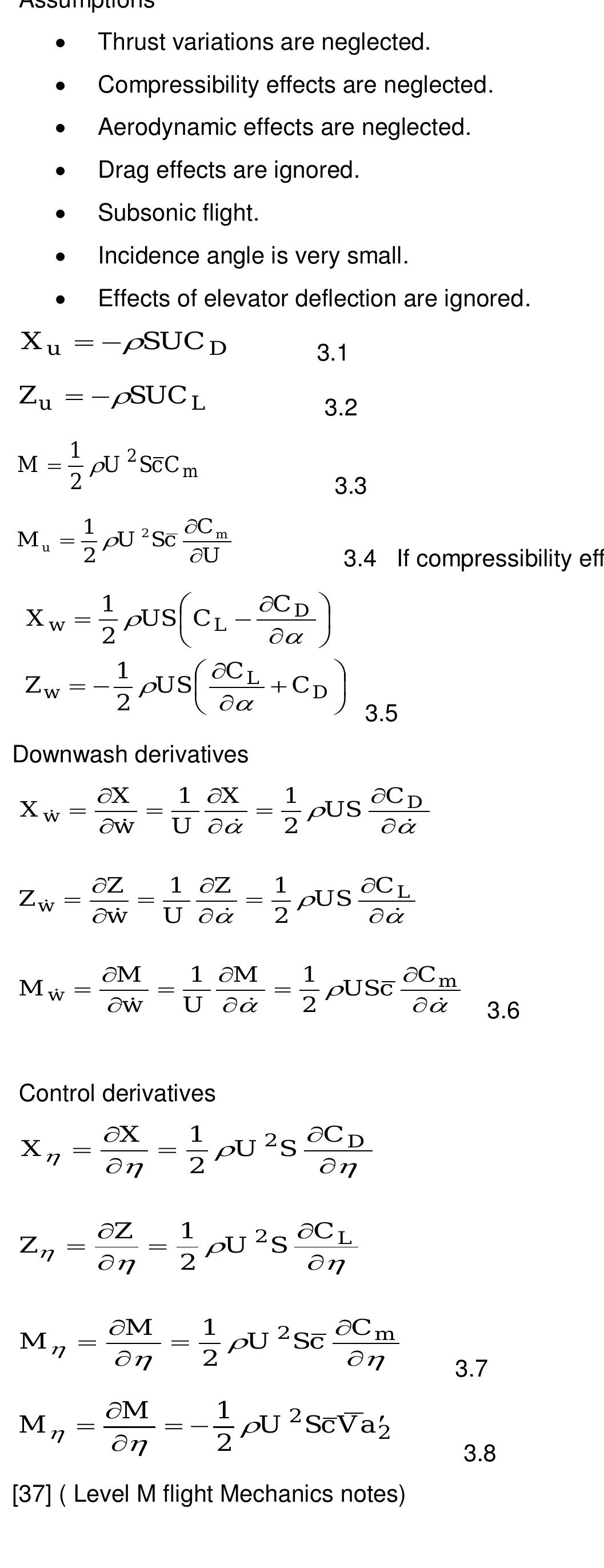X u   SUC D 3.1 Z u   SUC L 3.2 1 M  U 2 Sc C m 2 3.3 1 C m Mu  U 2 Sc 2 U 3.4 If compressibility effects are not ignored 1  C D  Xw  US  C L   2    1  C L  Zw   US   CD  2    3.5 Downwash derivatives X 1 X 1 C D   Xw   US w  U  2  Z 1 Z 1 C L   Zw   US w  U  2  M 1 M 1 Cm   Mw   USc w  U  2  3.6 Control derivatives X 1 C D X   U 2 S  2  Z 1 C L Z   U 2 S  2  M 1 Cm M   U 2 Sc  2  3.7 M 1 M    U 2 Sc V a2   2 3.8 [37] ( Level M flight Mechanics notes) Modelling and Simulation of a UH-UAV dynamics 14 School of Engineering and Technology *BEng Final Year Project Report Tail volume coefficients 3.9 3.10 Normal axis derivatives Normal force derivatives due to change in forward velocity, downwash, normal velocity, pitch rate and elevator deflection, respectively. 3.11 [38] Pitching moment derivatives 3.12 [39] 3.2.2 The Lateral Derivatives Yv , Lv , Lp , L , Nv , Np, Nr , N These derivatives are due to v, p, r, and disturbances The force causing the lateral motions is Y and the corresponding moments are L and N Lateral derivatives due to sideslip velocity (v) Yv: Derivative for change in lateral force due to change in sideslip velocity. Nv: Derivative for change in yawing moment due to change in sideslip velocity. Nv contribute to directional static stability. Nv >0 for a directionally stable UAV. Lv: Derivative for change in rolling moment due to change in sideslip velocity. Lv is important for roll stability. Lv< 0 for a roll stable UAV. [40] Modelling and Simulation of a UH-UAV dynamics 15 School of Engineering and Technology *BEng Final Year Project Report Lateral derivatives due to roll rate (p) Yp: Derivative for change in lateral force due to change in roll rate. Lp: Derivative for change in rolling moment due to rate of roll rate. Lp depends on wing area and size of tail surfaces. Np: Derivative for change in yawing moment due to rate of roll rate. Wing is the main contributor to Np. [41] Lateral derivatives due to yaw rate (r) Yr: Derivative for change in lateral force due to yaw rate. Nr: Derivative for change in yawing moment due to yaw rate. Nr is a yaw damping derivative. It is negative. Lr: Derivative for change in rolling moment due to roll rate. Lr is positive. Lateral derivatives due to aileron deflection Yξ: Derivative for change in lateral force due to change in aileron deflection. Lξ: Derivative for change in rolling moment due to change in aileron deflection. L ξ is a measure of aileron effectiveness. Nξ: Derivative for change in yawing moment due to aileron deflection. [Aerospace systems dynamics and control notes] Lateral derivatives due to rudder deflection Yζ: Derivative for change in lateral force due to rudder deflection. Lζ: Derivative for change in rolling moment due to rudder deflection. Nζ: Derivative for change in yawing moment due to rudder deflection. Nζ is a measure of rudder effectiveness. 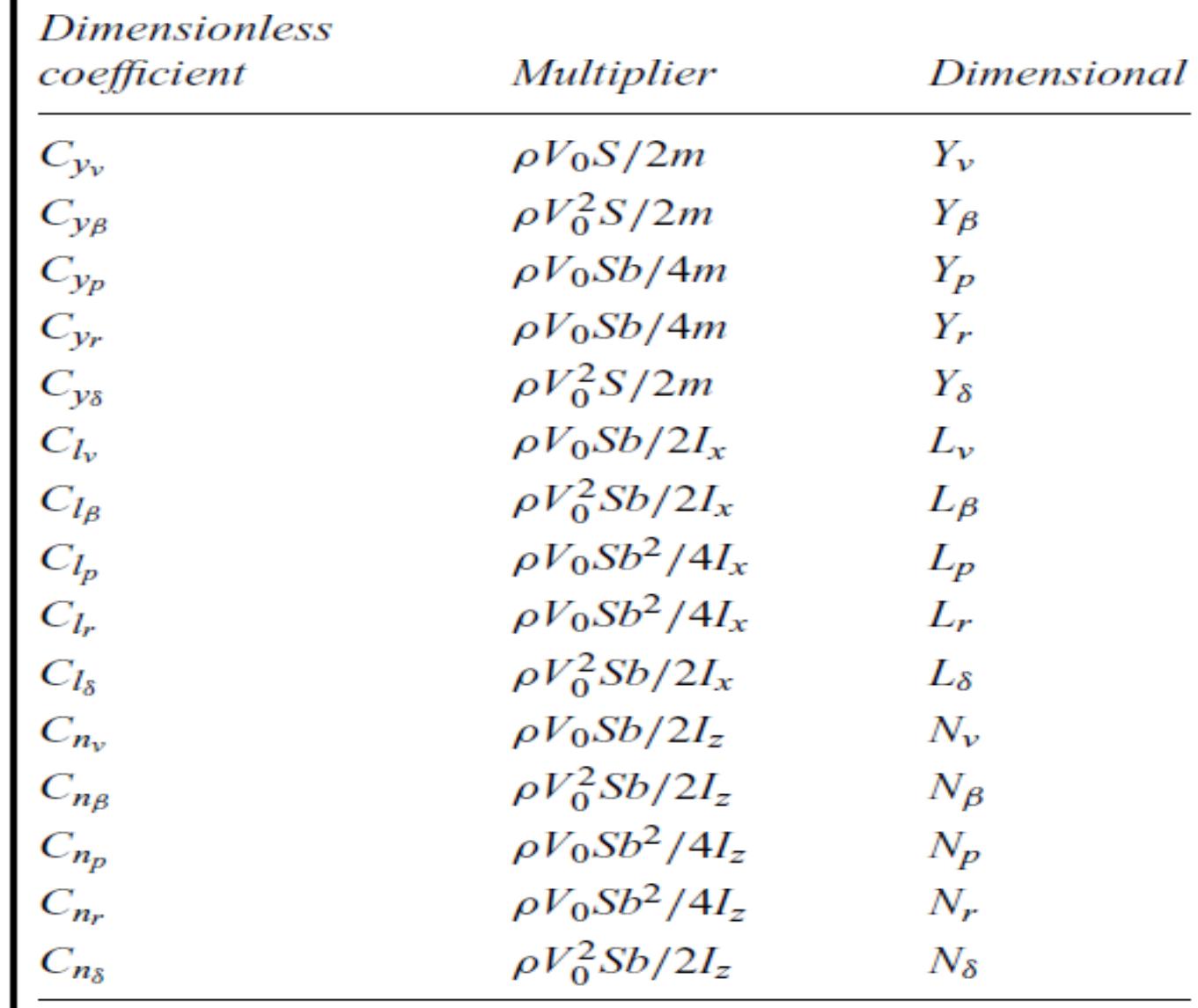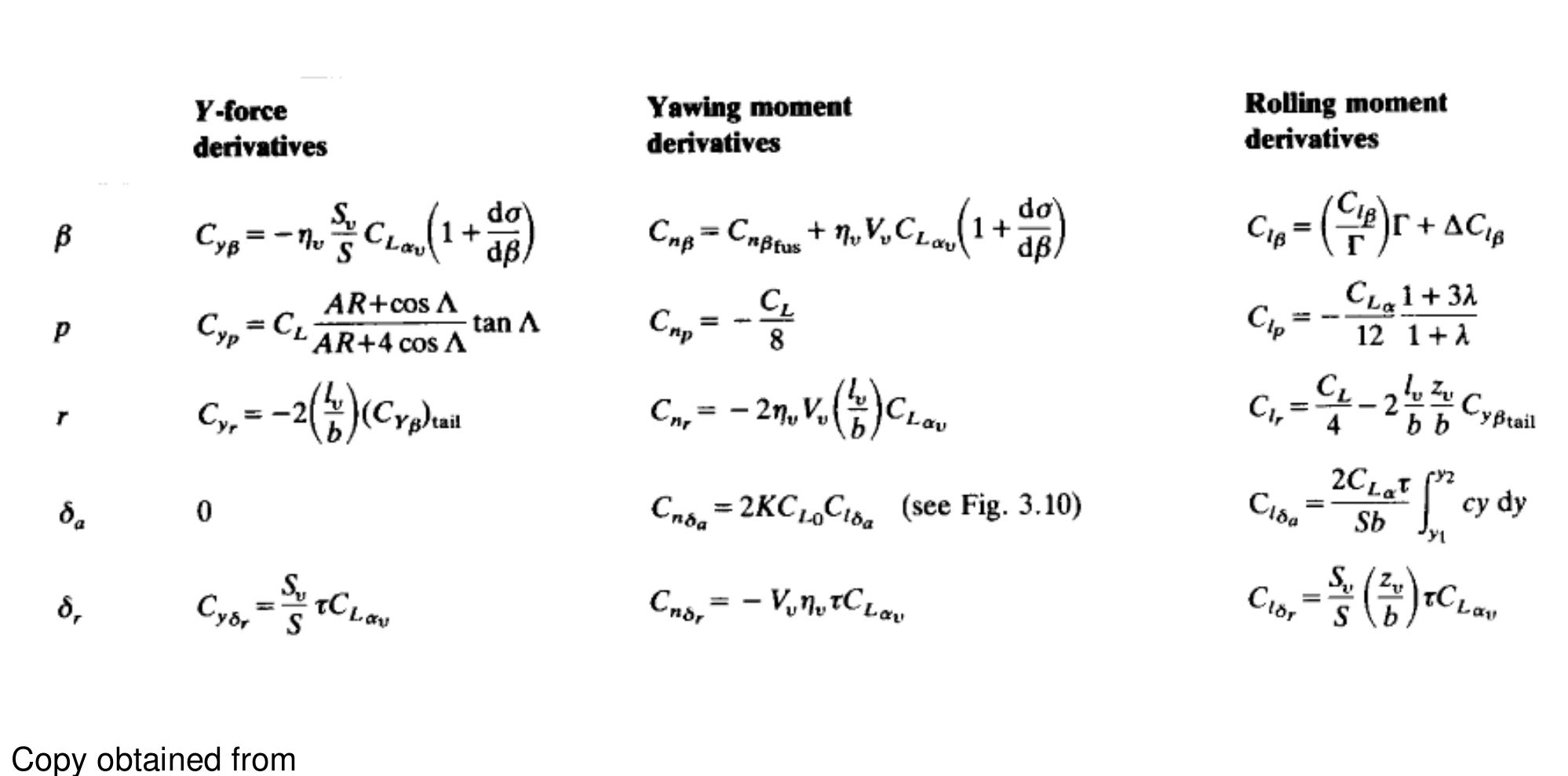[42] Rolling moment derivatives due to sideslip, roll rate, yaw rate and aileron deflection, respectively. 3.14 Modelling and Simulation of a UH-UAV dynamics 16 School of Engineering and Technology *BEng Final Year Project Report Yawing moment derivatives due to sideslip, roll rate, yaw rate and rudder deflection, respectively 3.15 [43] Lateral force derivatives due to sideslip, roll rate, yaw rate and rudder deflection 3.16 3.17 3.18 [44] 4 UAV Longitudinal motions Assuming stick fixed The longitudinal motions to be analysed is the short pitching period oscillation (SPPO) and the phugoid motion. SPPO is a highly damped motion characterised by change in incidence angle and pitch angle in phase at constant forward speed. Assuming u=0 [45], (Introduction to aircraft stability and control 2 ASE4 notes studynet ) Estimating UAV SPPO 4.1 [46] Mq is the derivative for pitching moment due to pitch rate Mα,Mά are the derivative for pitching moment due to change in incidence Zα is the derivative for change in normal force due to incidence Uo is change in forward speed Modelling and Simulation of a UH-UAV dynamics 17 School of Engineering and Technology *BEng Final Year Project Report 4.2 Period = 2π/ω t1/2= -ln2/(-ζωn) time to half amplitude N1/2 = (t1/2)/Period, number of cycles Phugoid Phugoid is the lightly damped oscillation with a long period. It is characterised by change in pitch attitude angle with very small changes in incidence. The change in forward speed is out of phase with pitch attitude angle by 90°. [47], (Introduction to aircraft stability and control 2 ASE4 notes studynet ) Estimating UAV phugoid 4.3 Xu and Zu are derivatives due to forward speed Uo is the forward speed g is the acceleration due to gravity Estimation of phugoid 4.4 Period = 2π/ω t1/2= -ln2/(-ζωn) , time to half amplitude N1/2 = (t1/2)/Period, number of cycles [48] 4.1 Derivative influence on longitudinal motion The characteristic equations show clearly the influence of derivatives to the longitudinal motion. If the damping ratio and the frequency of the SPPO motion is high; the UAV will have a faster response to elevator input without overshoot. However if the UAV has lightly damped motion with low frequency, the UAV will be difficult to control. [49] Influence of stability derivatives of longitudinal motions Mq and Mά these are SPPO damping derivatives . Increasing Mq and Mά increases the damping of the SSPO motion. Mα is the SPPO frequency derivative. Increasing Mα increases the frequency of the SPPO motion. Xu is the damping derivative for phugoid motion. Increasing Xu increases the damping ratio of the phugoid motion. Modelling and Simulation of a UH-UAV dynamics 18 School of Engineering and Technology *BEng Final Year Project Report Zu is the derivative for the frequency of the phugoid motion. Increasing Zu increases frequency of the phugoid motion. The UAV should be easy to control therefore it should be designed to have heavily damped motions with high frequency. Therefore the Mα, Mά and Mq derivatives should be large. [50] 5 UAV Lateral motion Assuming stick fixed The lateral motions to be simulated and analysed are Directional divergence, Spiral divergence and Dutch roll oscillation. These are characterised by a combination of rolling, yawing and sideslip motions. [51] Roll mode Heavily damped none oscillatory motion. A roll disturbance will cause an up-going wing to decrease in lift while the down-going wing increases in lift. This develops a restoring rolling moment that damps out the motion. However the UAV does not return to its original position. [52], (Introduction to aircraft stability and control 2 ASE4 notes studynet ) Estimating UAV roll mode Characteristic equation 5.1 τ is roll time constant. ζr = Lp t1/2 = -ln2/Lp Spiral A side slip disturbance will cause a yawing moment due to fin, this will result a yawing motion which develops a rolling moment. The rolling moment then causes an increase in sideslip velocity. [53], (Introduction to aircraft stability and control 2 ASE4 notes studynet) Estimating UAV spiral mode. Assuming the derivatives has the usual signs. That is ignoring control reversal. The characteristic equation 5.2 The condition for stable spiral mode 5.3 [54] Modelling and Simulation of a UH-UAV dynamics 19 School of Engineering and Technology *BEng Final Year Project Report Dutch roll mode An oscillatory motion resulting from a disturbance in yaw, there is a restoring yawing moment and damping force due to fin. This is a very undesirable motion. Estimating UAV Dutch roll mode 5.4 Characteristic equation 5.5 Damping and frequency for the Dutch roll motion 5.6 Period = 2π/ω 5.7 t1/2= -ln2/(-ζωn) time to half amplitude 5.8 N1/2 = (t1/2)/Period, number of cycles 5.9 [55] 6 Models and Simulations Matlab and Simulink is a technical computing language which was used to model the UAV and simulate its dynamics. 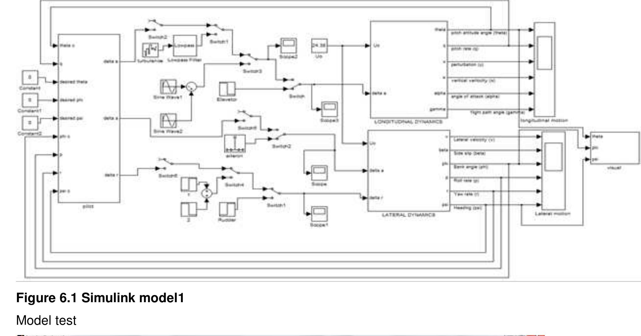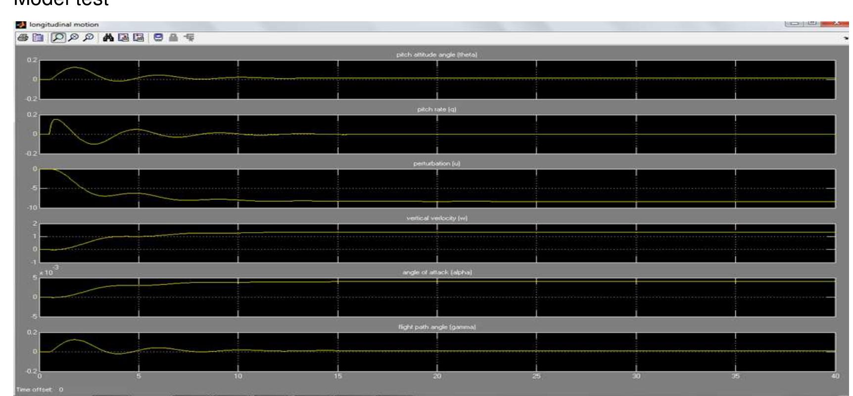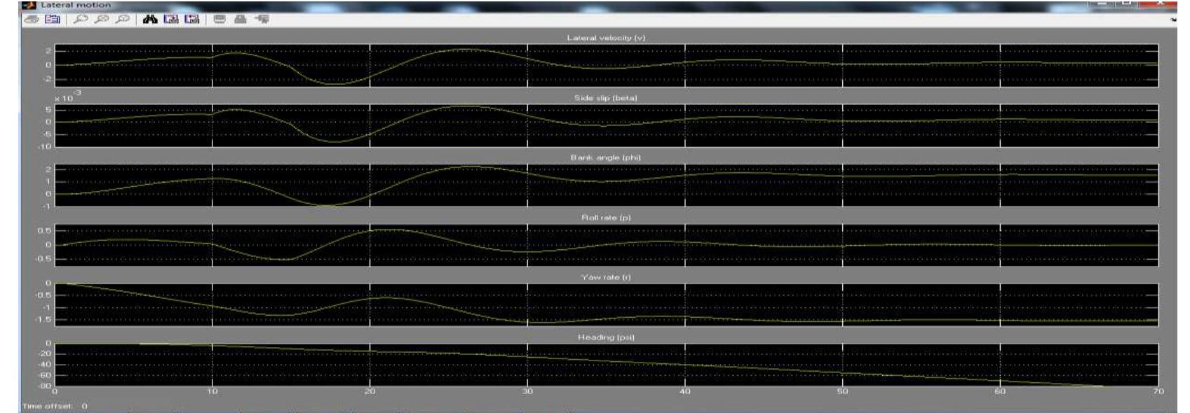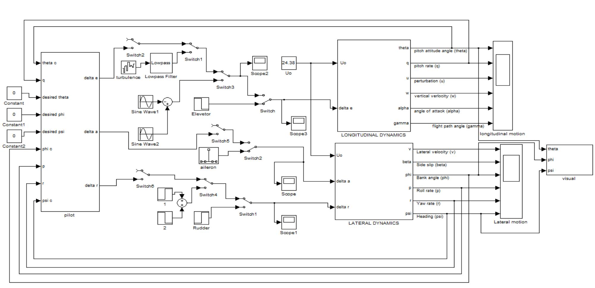A generic Simulink model was created to simulate the UAV dynamics. The model was then tested using the Navion aircraft derivatives. The Navion aircraft was used because a lot of simulation results and its dynamics characteristics are readily available. The data is available online and in textbooks such as Flight stability and Automatic control by Robert C Nelson. The derivatives were computed to determine the forces and moments. The inputs to the model were the control surfaces and the atmospheric disturbances. 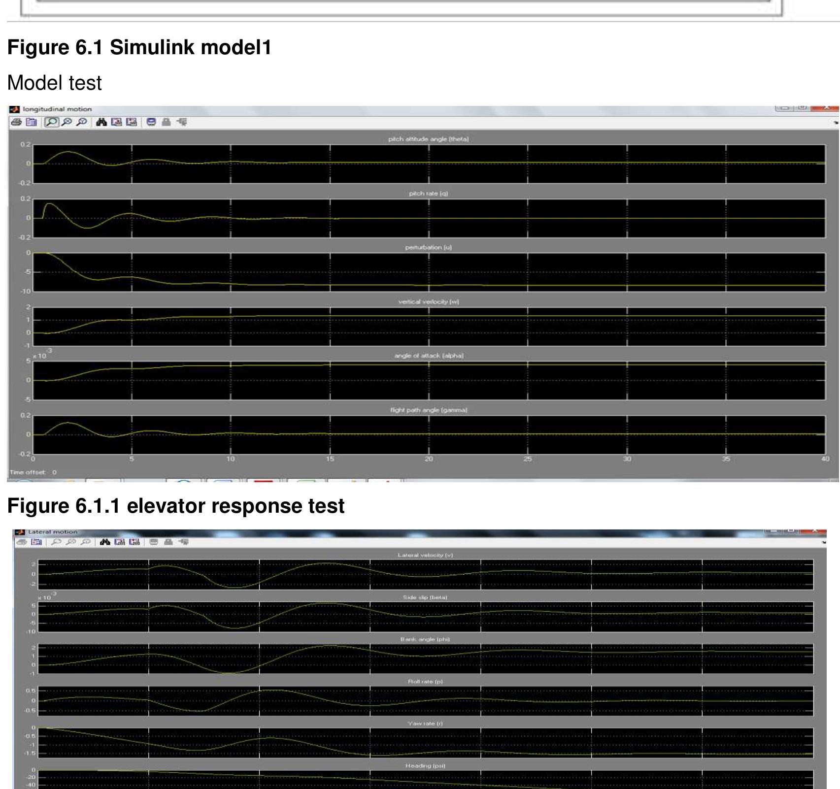The outputs of the model were the angles and rates; [Figure 6.1.1]. The model has a visual platform with Matlab based animation and flight gear interface using UDP protocol. The autopilot block provides a platform for flight augmentation, if required. The derivatives are specific for the specified flight condition. That is speed and altitude. Therefore the simulation can only be run for a single flight speed. Each time the flight condition changes the whole derivatives would have to be calculated again. The wind gust and wind shear magnitude and direction cannot be specified accurately. These are some of the major drawbacks of the model. Hence an alternative model had to be developed. 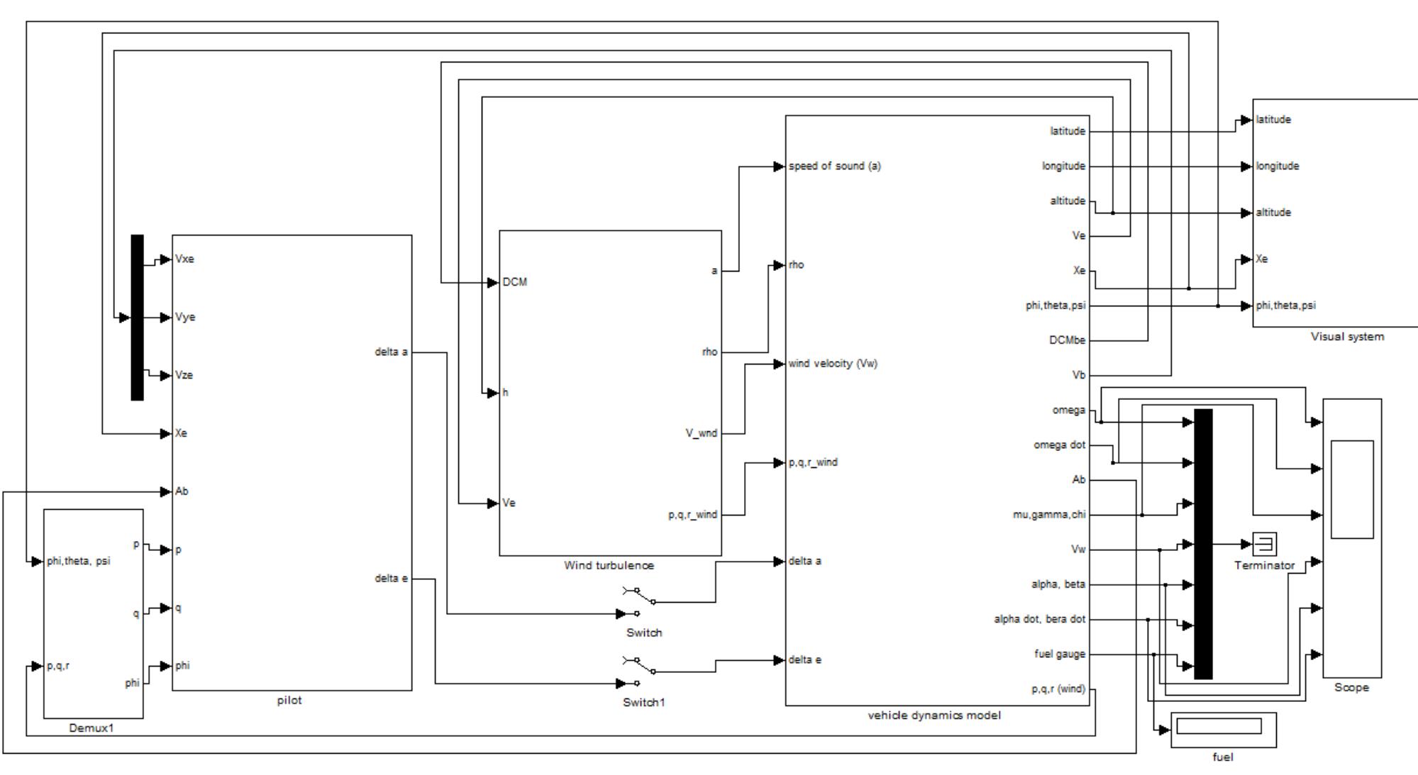Modelling and Simulation of a UH-UAV dynamics 20 School of Engineering and Technology *BEng Final Year Project Report 6.1 The UAV generic model 1 Figure 6.1 Simulink model1 Model test Figure 6.1.1 elevator response test Figure 6.1.2 rudder response test Modelling and Simulation of a UH-UAV dynamics 21 School of Engineering and Technology *BEng Final Year Project Report 6.2 UAV generic model 2 Further work was done to develop a model that can simulate the whole flight profile. The model does not require change of derivatives. This is achieved by use of digital datcom. The datcom is linked to the Simulink model and it estimates the derivatives at different altitudes and flight speeds based on the UAV geometry. The model has a wind shear, turbulence and gust platform, where the wind speed and direction can be changed to analyse its effects on the UAV. The models combine both wind and body axis system. There is a visual platform for Matlab based animation, flight path data and an interface with flight gear. This enables the user to visually analyse the dynamics of the UAV. The model also has a flight augmentation platform for when it is required. The models also have extra benefits such as mission profile analysis, endurance test, testing what is and not possible for the UAV in terms of extreme bank angle, turn rate, etc depending on the speeds. The digital datcom is usually programmed in FORTRAN language. It takes time to understand how it works and need someone who really knows the program. Errors in the dtacom program might go unnoticed and this further limits the reliability of the model as a whole; hence a major drawback. However the benefits outweigh the drawbacks hence the model can be used for UAV dynamics analyses. A solution for both model 1 and model 2 drawbacks was required. A general solution to all drawbacks of both models was developed. Generic model 2 Figure 6.2 Simulink model 2 This was the solution to drawbacks highlighted in model1 Modelling and Simulation of a UH-UAV dynamics 22 School of Engineering and Technology *BEng Final Year Project Report 6.3 UAV generic model 3 The solution was as a result of the group members not providing data required for the simulation. The wind tunnel test had not been carried out and the computational fluid dynamics analyses (CFD) was not completed. 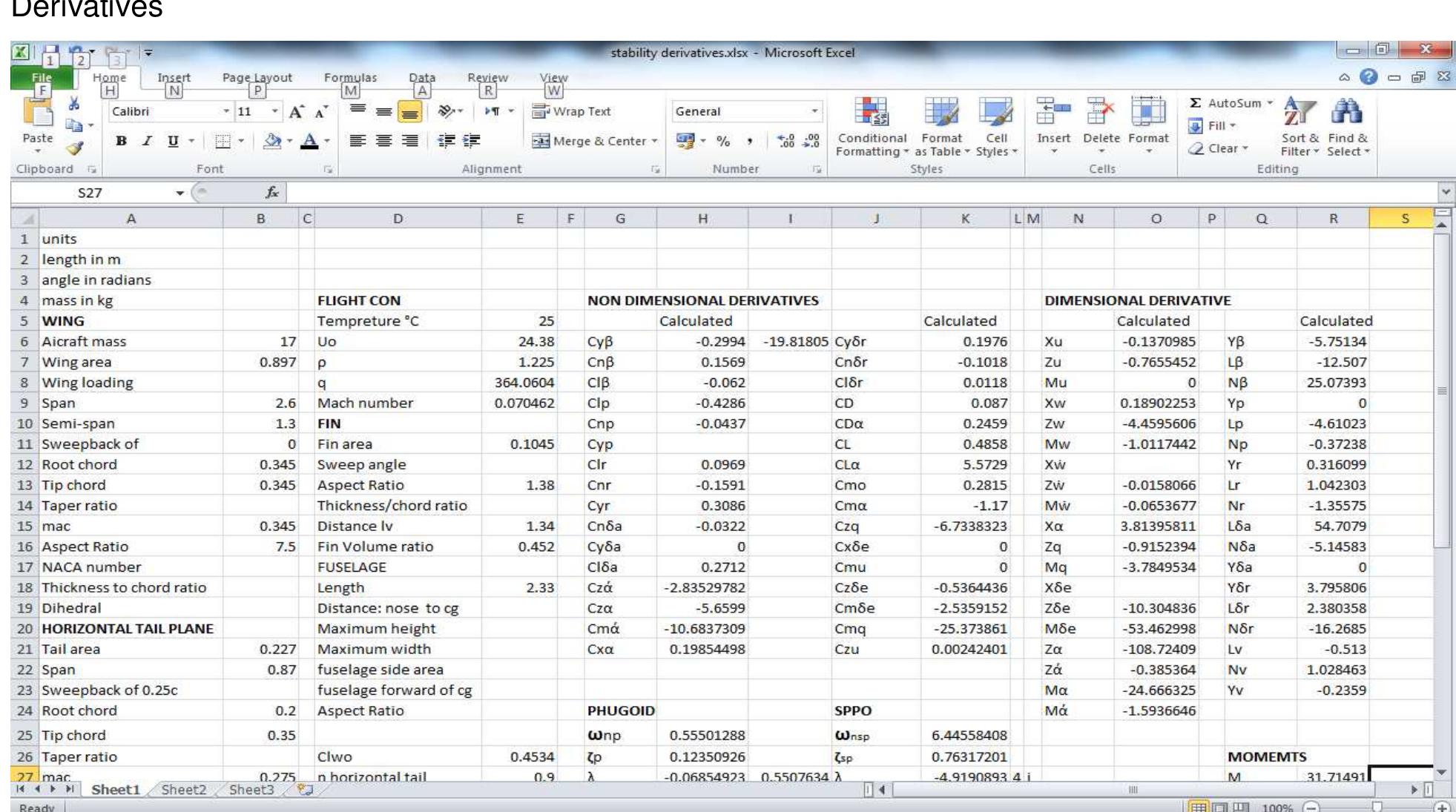The structural designer was not providing the values required to estimate the derivatives. Therefore a solution was to use an excel file that calculates all the derivatives based on the geometry and flight condition. The data from the wind tunnel and CFD would be entered once available. The file estimates all the required derivatives for an accurate analysis of the dynamics. It also estimates the frequency and damping for spiral mode, dutch roll mode, roll mode, pure yaw motion, SPPO and phugoid. The model also estimates X,Y,Z forces and the M,N,L moments. 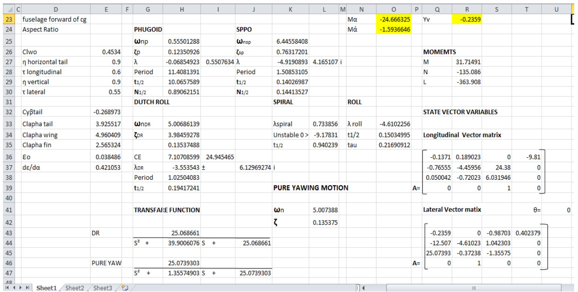The longitudinal and lateral transfer functions and Eigen vectors for wind shear and motions can be obtained from the model3, [Figure 6.3.3]. When the speed is changed the derivatives, motions, forces and moments automatically updates. This saves time by not having to recalculate all the derivatives each time the flight condition changes, [Figure 6.3.1]. This model offers far more benefits with potential for further development. Effects of changing the UAV geometry on motions can be analysed. This allows flexibility on testing various geometries and finding the most suitable UAV geometry for the intended mission. Mathworks has interfaced with Microsoft applications. Therefore lookup Simulink function blocks can be used to directly source data from the excel model. This solves the Simulink model 1 drawback because changing speed or geometry of the UAV in excel file will automatically updates the Simulink model 1. The excel model will allow the Simulink model 1 to be flexible and saves a lot of time. Linking Simulink model1 and excel model will increase chances of failure in Simulink model 1 but it’s a minor drawback considering the benefits. The excel file is easy to update; it does not require much knowledge to change geometry values and input new UAV model. This saves time and also the estimates for motions, forces and moments can be compared to the outputs of Simulink model 2; thus solving the model 2 drawbacks. The excel model can further be developed to include irritation functions. This allows the designer to choose the frequency and damping of the motions and the model will output a suggested geometry by changing tail area, wing area, chord, span, tail position from cg, dihedral angle etc. The equations used for the model calculations are listed in Appendices. 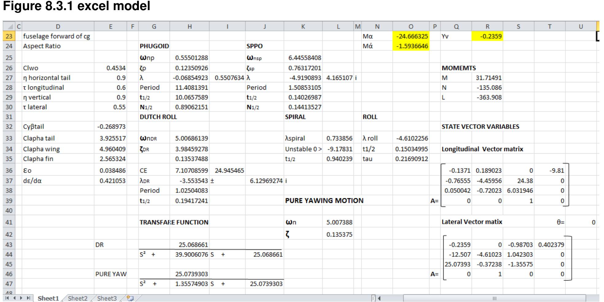Modelling and Simulation of a UH-UAV dynamics 23 School of Engineering and Technology *BEng Final Year Project Report UAV model 3 Derivatives Figure 6.3.1 Excel model Motion and forces , Eigen vectors and transfer functions Figure 6.3.2 Excel model Modelling and Simulation of a UH-UAV dynamics 24 School of Engineering and Technology *BEng Final Year Project Report 7 Results MAK II is a UH UAV. MAK II geometry was used for the simulation. The damping ratio (ζ) and the undamped frequency (ω) was calculated using the excel model. Time period, time to half amplitude and the number of cycles was also determined using the excel model. This was then used to validate the Simulink model. 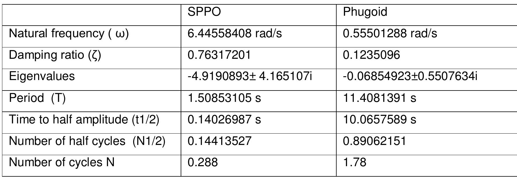7.1 Longitudinal dynamics The long term (phugoid) and short term (SPPO) dynamics of step elevator input Table 1 Longitudinal motion SPPO Phugoid Natural frequency ( ω) 6.44558408 rad/s 0.55501288 rad/s Damping ratio (ζ) 0.76317201 0.1235096 Eigenvalues -4.9190893± 4.165107i -0.06854923±0.5507634i Period (T) 1.50853105 s 11.4081391 s Time to half amplitude (t1/2) 0.14026987 s 10.0657589 s Number of half cycles (N1/2) 0.14413527 0.89062151 Number of cycles N 0.288 1.78 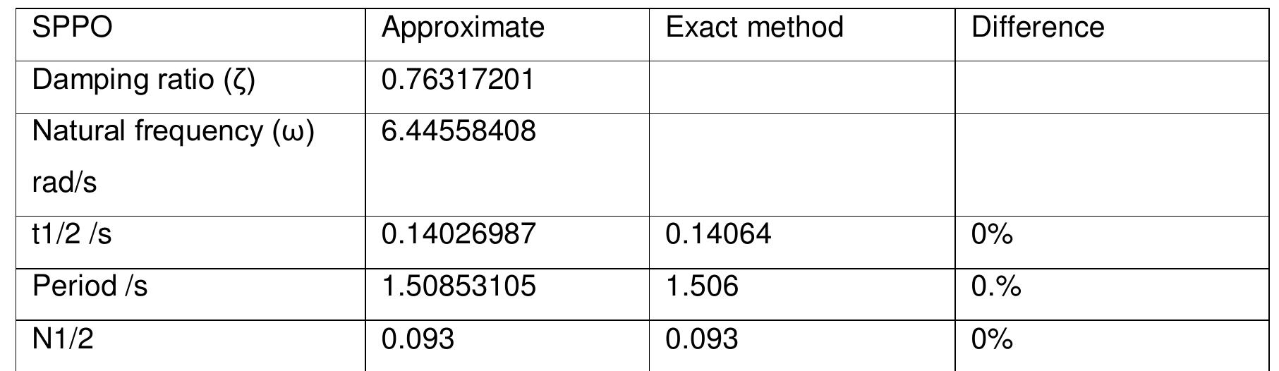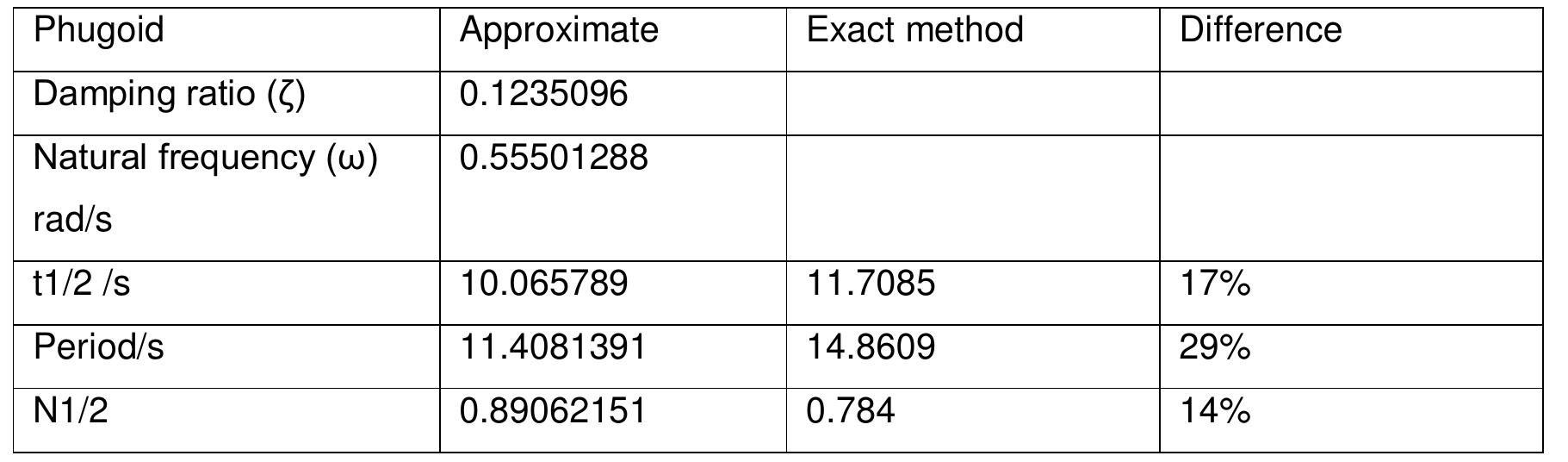The table above shows that the phugoid motion damps half of its initial amplitude in approximately 10 seconds. The phugoid motion lasted around 2 cycles. The SPPO motion lasted for 0.3 cycles. 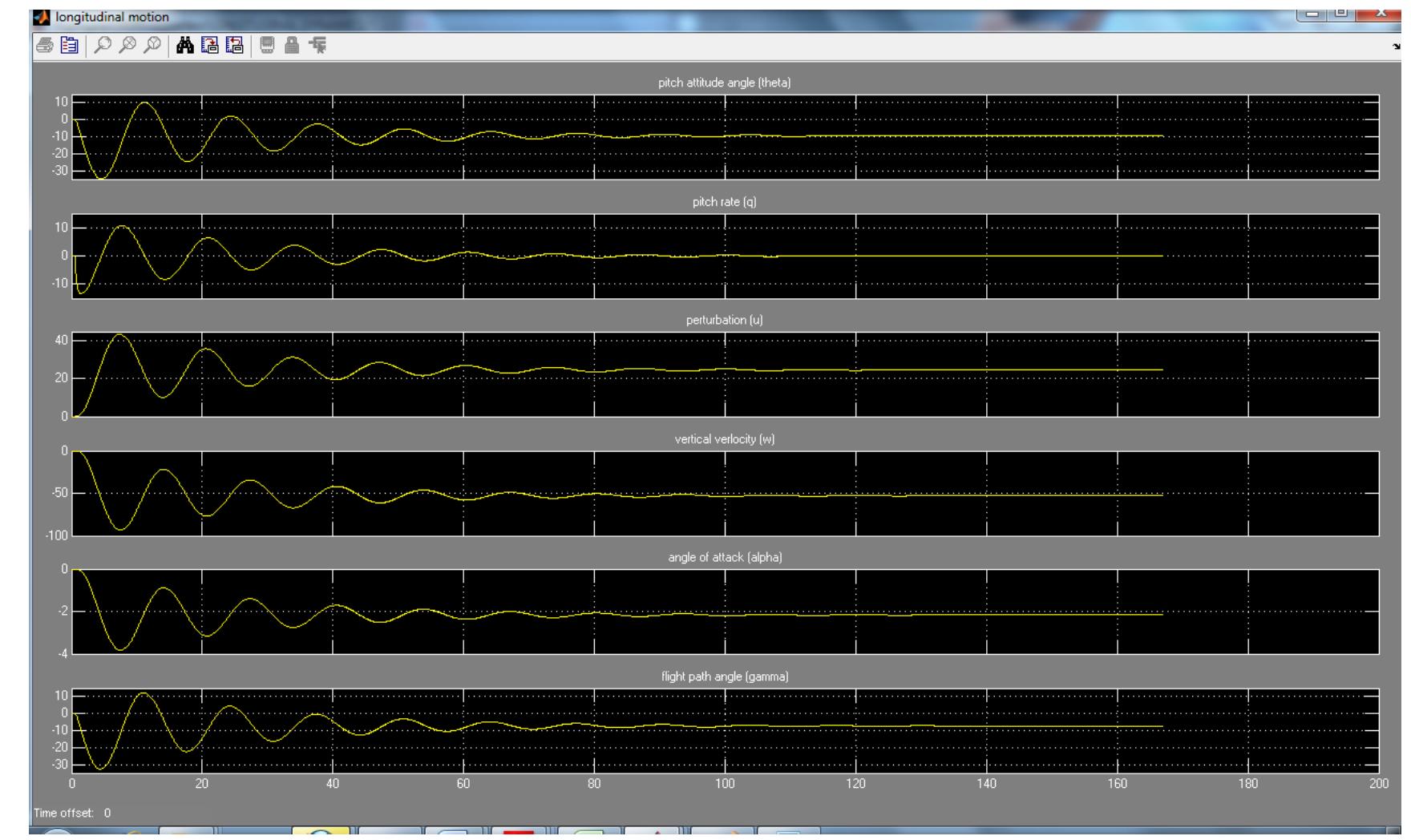Modelling and Simulation of a UH-UAV dynamics 25 School of Engineering and Technology *BEng Final Year Project Report Long-term response Simulink model Figure 7.1.1 Long term response to elevator step input The figure above shows that the UAV returns to equilibrium position in approximately 80 seconds after an elevator step input disturbance. This shows that the UAV longitudinal dynamics are stable. The pitch rate (q) returns to zero steady state from a maximum pitch rate of 9°/s. The angle of attack (α) has decreased by 2° due to the influence of SPPO mode. 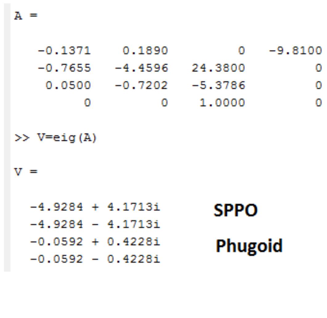The excel model was used to obtain an Eigen vector. The Eigen vector was then solved in Matlab to obtain the Eigen values. Modelling and Simulation of a UH-UAV dynamics 26 School of Engineering and Technology *BEng Final Year Project Report Table 2 SPPO comparison SPPO Approximate Exact method Difference Damping ratio (ζ) 0.76317201 Natural frequency (ω) 6.44558408 rad/s t1/2 /s 0.14026987 0.14064 0% Period /s 1.50853105 1.506 0.% N1/2 0.093 0.093 0% Table 3 phugoid comparison Phugoid Approximate Exact method Difference Damping ratio (ζ) 0.1235096 Natural frequency (ω) 0.55501288 rad/s t1/2 /s 10.065789 11.7085 17% Period/s 11.4081391 14.8609 29% N1/2 0.89062151 0.784 14% 7.2 UAV responds to Gust and turbulence 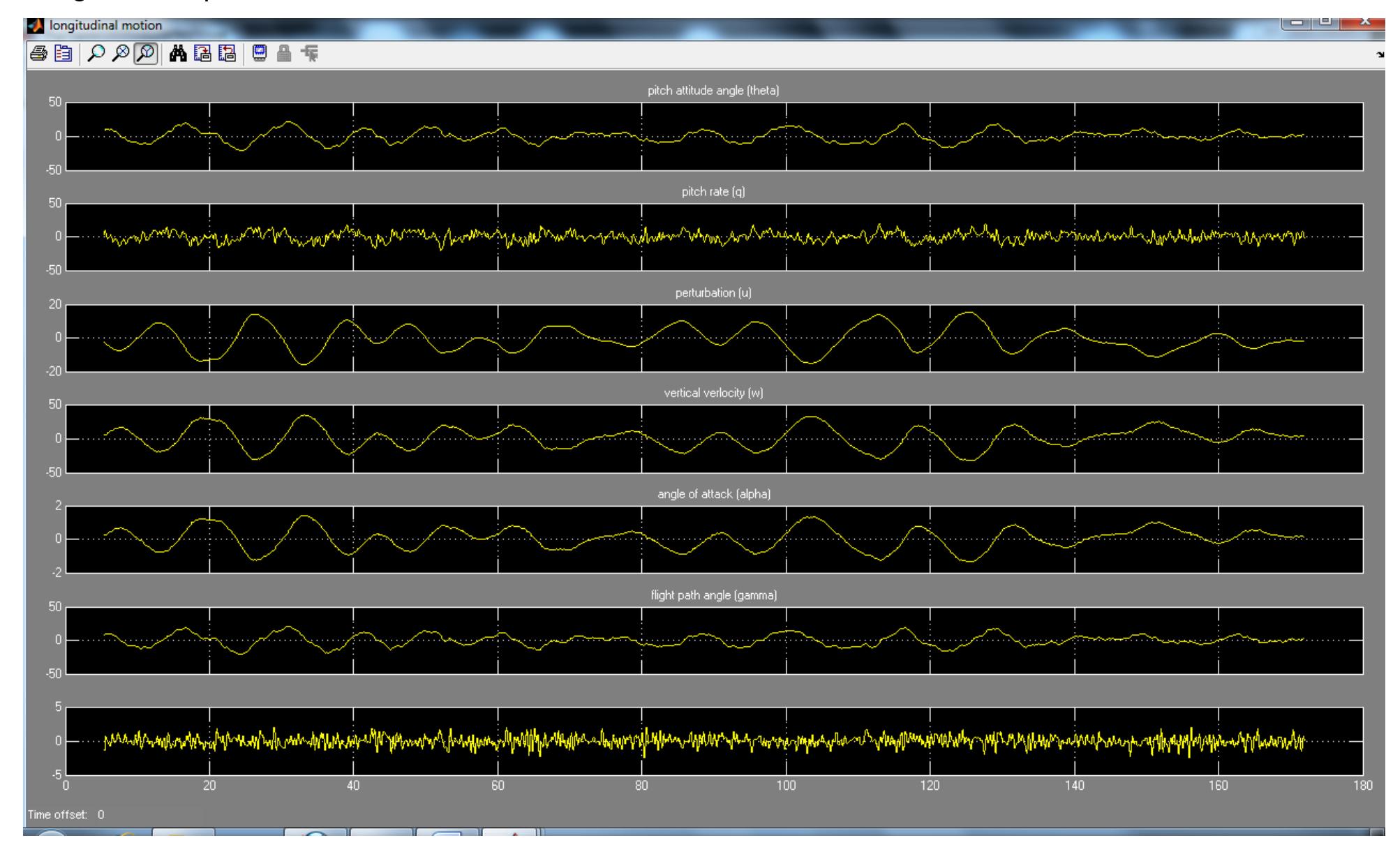Turbulence is a chaotic system. It’s not liner and cannot be mathematically predicted. Therefore noise generator was used to generate the turbulence and a low pass filter to determine the amplitude of the turbulence. Sine waves can be used to characterise sinusoidal gust. The turbulence was assumed to be a stationary phase that the UAV flies through. The effects of the turbulence on the UAV dynamics are increased by increasing the turbulence speed and amplitude. The UAV was subjected to various turbulent profiles and it exhibited positive dynamic stability characteristics, [Figure 7.2]. The wind shear vector can be obtained from the excel model, [APPENDIX C]. The effects of wind shear to the longitudinal model can then be analysed based on the Civil Aviation Organisation (ICAO) standards. [56] The knowledge of UAV’s response to wind shear and turbulence is useful when setting the limiting flight conditions at which the UAV can be flown. Avoiding extreme flight conditions may result in reduced maintenance cost and longer life cycle for the UAV. Modelling and Simulation of a UH-UAV dynamics 27 School of Engineering and Technology *BEng Final Year Project Report Long-term response to turbulence Figure 7.2 response to turbulence 7.3 Lateral Dynamics The excel model was used to estimate the lateral motions. These were then used to validate the Simulink model. Matlab was used to obtain Eigen values from excel Eigen vectors for the exact method. Modelling and Simulation of a UH-UAV dynamics 28 School of Engineering and Technology *BEng Final Year Project Report Table 4 Roll mode Approximate Exact Difference Eigenvalue -4.6102256 -4.822 4.5% Time constant Estimated 0.21690912 s Observed 6.3 s t1/2 0.15034995 s 0.1437s 4.4% Table 5 Spiral mode Approximate Exact Difference Eigenvalue 0.733856 0.0293 Stability criteria 0>-9.17831 Unstable! [0<(LβNr>NβLr)] t2 0.940239s 23.7s Huge difference! 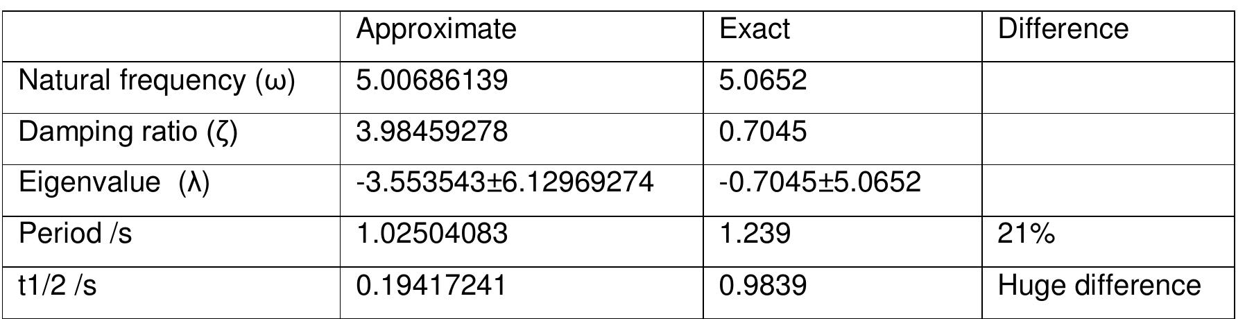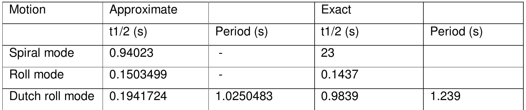Table 6 Dutch role mode Approximate Exact Difference Natural frequency (ω) 5.00686139 5.0652 Damping ratio (ζ) 3.98459278 0.7045 Eigenvalue (λ) -3.553543±6.12969274 -0.7045±5.0652 Period /s 1.02504083 1.239 21% t1/2 /s 0.19417241 0.9839 Huge difference Table 7 exact and approximate comparison Motion Approximate Exact t1/2 (s) Period (s) t1/2 (s) Period (s) Spiral mode 0.94023 - 23 Roll mode 0.1503499 - 0.1437 Dutch roll mode 0.1941724 1.0250483 0.9839 1.239 Modelling and Simulation of a UH-UAV dynamics 29 School of Engineering and Technology *BEng Final Year Project Report Long-term lateral response to roll disturbance 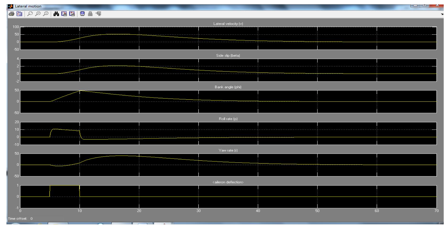Figure 7.3.1 UAV aileron ipulse input response The long-term response [Figure 7.3.1] shows that the MAK2 UH-UAV has positive lateral dynamic stability. The UAV settles to zero steady state in 30s after a roll disturbance. There is no overshoot, hence a heavily damped. This correspond predicted roll mode [Table 4] Long-term lateral response to rudder step input. 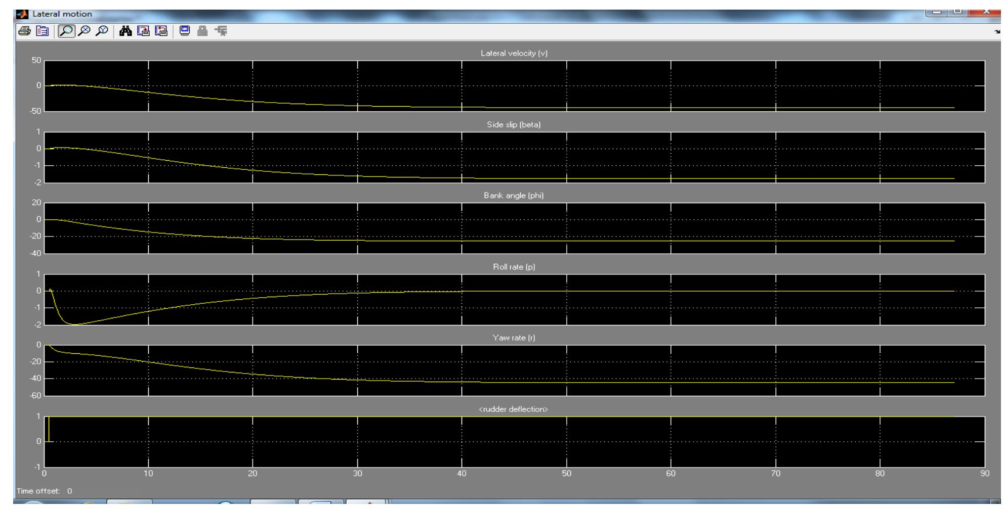Figure 7.3.2 UAV rudder step input response The figure 7.3.2 above shows a rudder step input response. The UAV reached a steady state in 35s. The UAV will not return to its original sate because the rudder is left deflected. 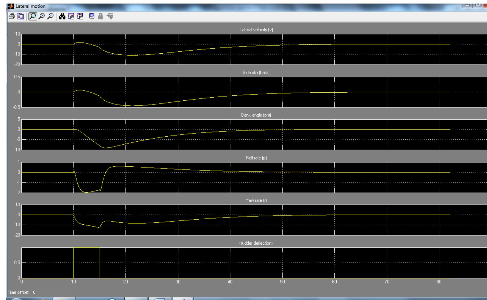Modelling and Simulation of a UH-UAV dynamics 30 School of Engineering and Technology *BEng Final Year Project Report Long-term response to lateral disturbance Figure 7.3.4 UAV response to yaw disturbance 8 The UAV Simulink models This section will further analyse the Simulink model components and how they work. 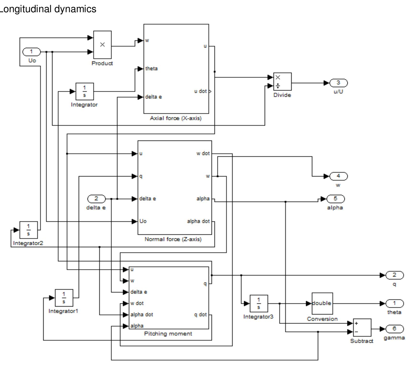8.1 Simulink Model 1 Figure 8.1.1 model 1 Modelling and Simulation of a UH-UAV dynamics 31 School of Engineering and Technology *BEng Final Year Project Report Longitudinal dynamics Figure 8.1.2 longitudinal dynamics The longitudinal dynamics are calculated in the longitudinal dynamics platform. This comprises of the axial force, Normal force and pitching moment subsystems. The angles, rates and velocities are calculated in the subsystems. 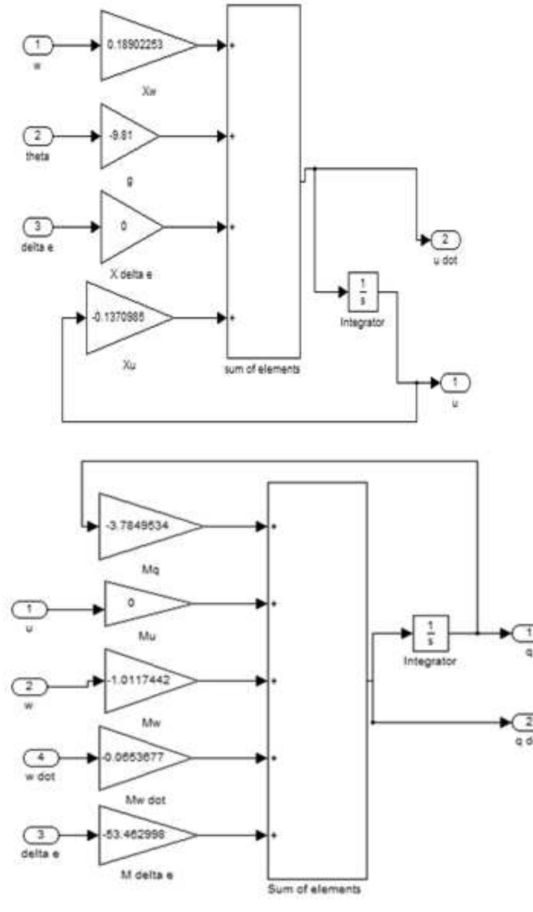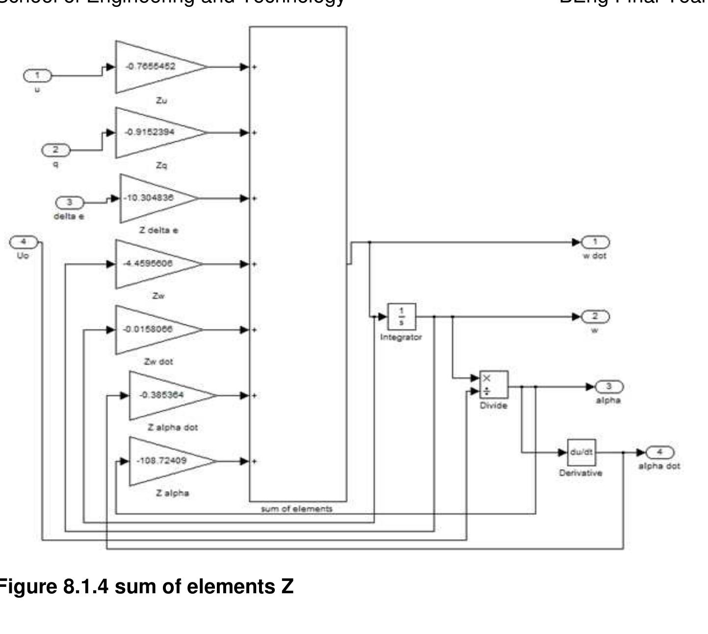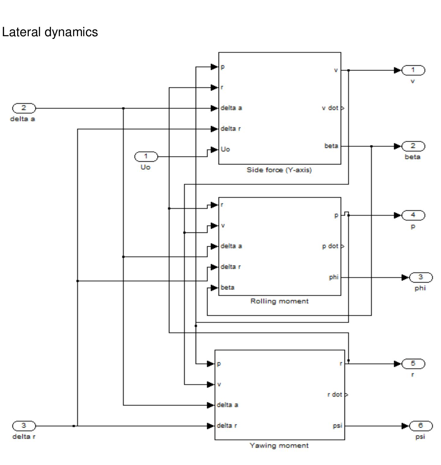Modelling and Simulation of a UH-UAV dynamics 32 School of Engineering and Technology *BEng Final Year Project Report Figure 8.1.3 sum of elements X and M Modelling and Simulation of a UH-UAV dynamics 33 School of Engineering and Technology *BEng Final Year Project Report Figure 8.1.4 sum of elements Z Lateral dynamics Figure 8.1.5 Lateral dynamics Modelling and Simulation of a UH-UAV dynamics 34 School of Engineering and Technology *BEng Final Year Project Report The lateral dynamics are calculated in the lateral dynamics platform. This comprises of the side force, rolling and yawing moment subsystems. 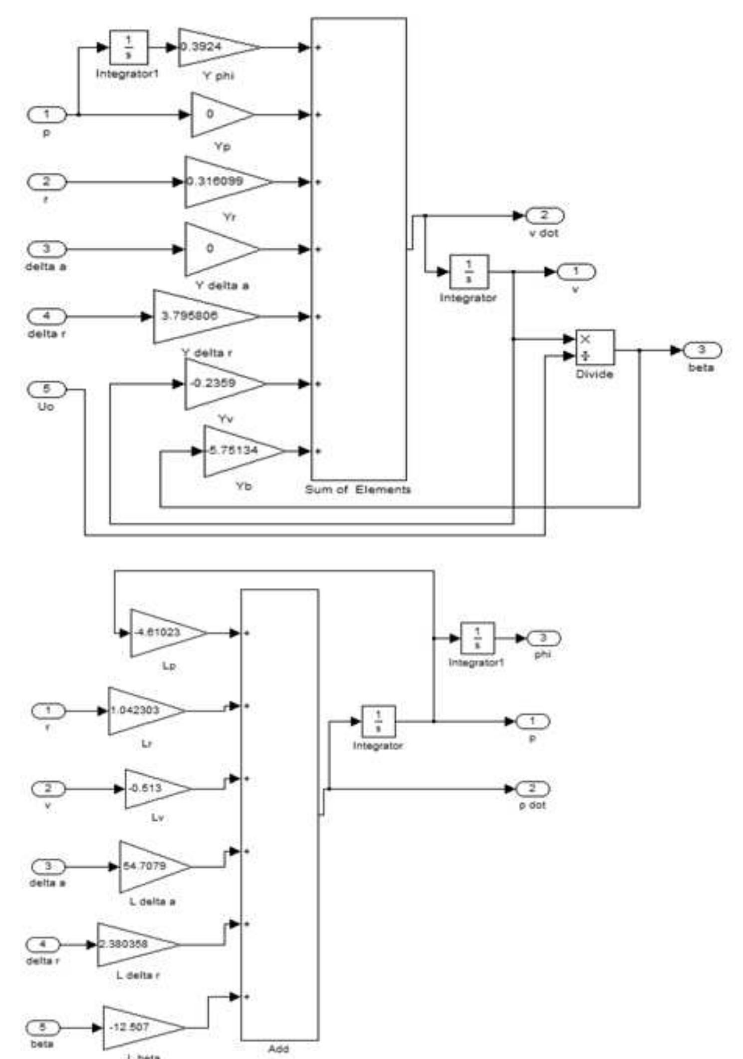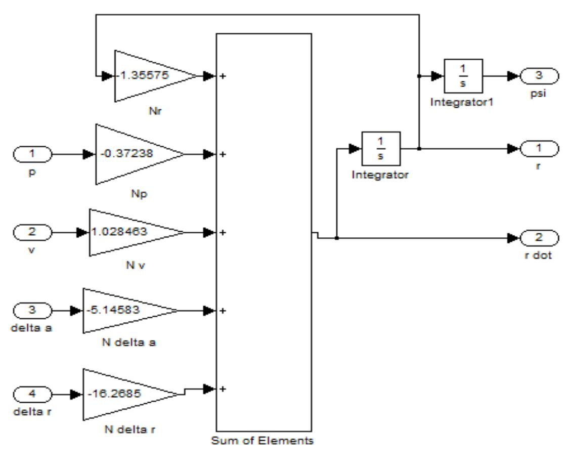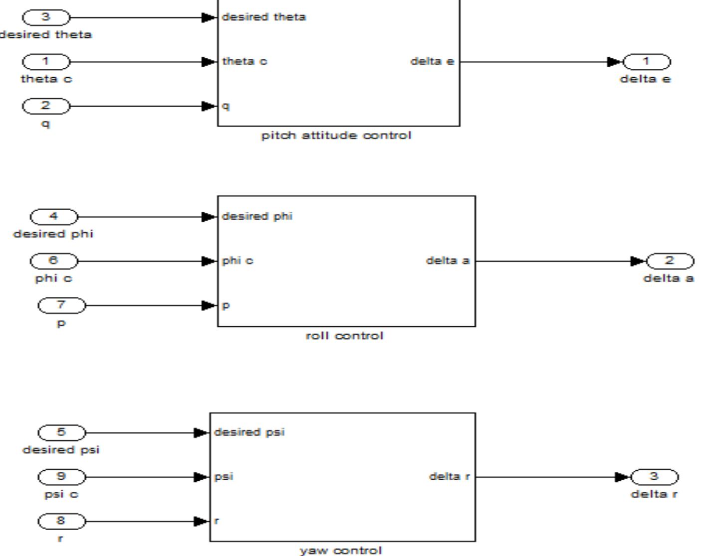The force and moments subsystems Figure 8.1.6 sum of elements Y and L Modelling and Simulation of a UH-UAV dynamics 35 School of Engineering and Technology *BEng Final Year Project Report Figure 8.1.7 sum of elements N Augmentation A feedback system can be introduced to the system by using the pilot platform. The control subsystem contains gyroscope, accelerometer gains and servo actuators. 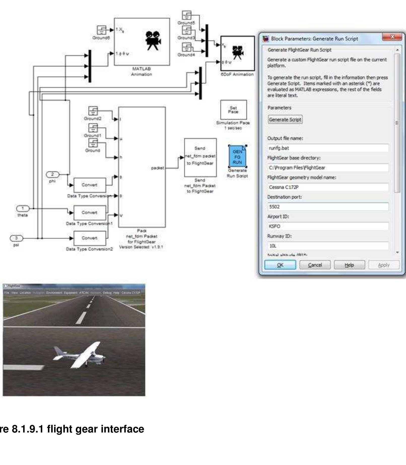Figure 8.1.8 control platform Modelling and Simulation of a UH-UAV dynamics 36 School of Engineering and Technology *BEng Final Year Project Report Visual platform This is the flight gear interface and Matlab based animation. 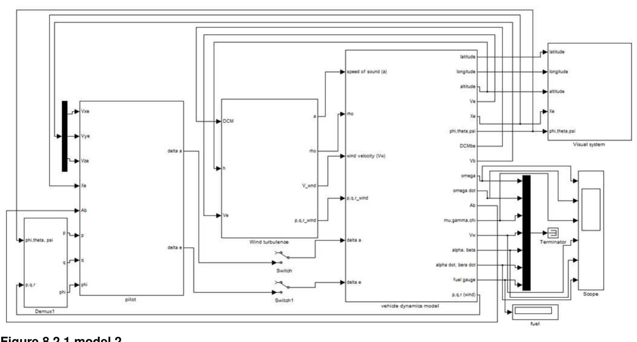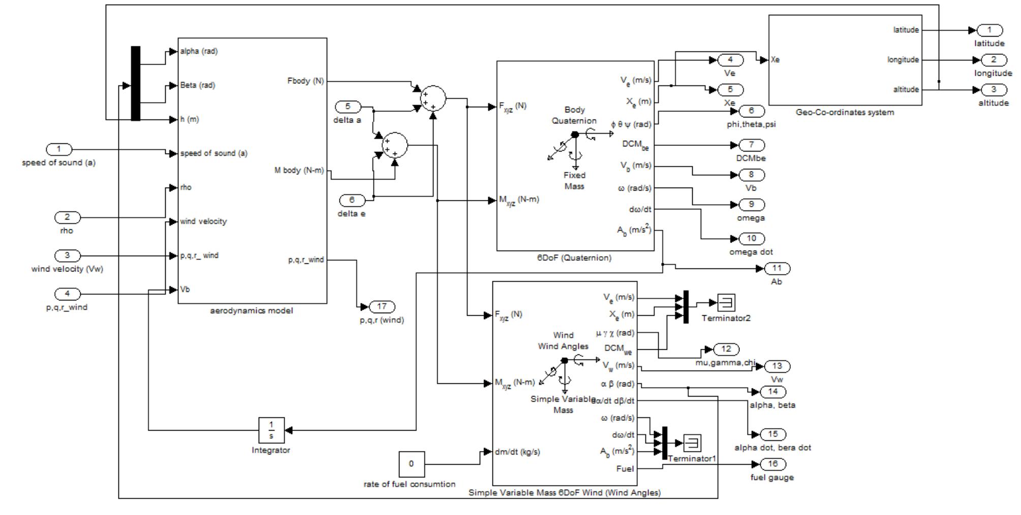Figure 8.1.9.1 flight gear interface Modelling and Simulation of a UH-UAV dynamics 37 School of Engineering and Technology *BEng Final Year Project Report 8.2 Simulink model 2 Figure 8.2.1 model 2 The longitudinal and lateral dynamics are calculated in the vehicle dynamics platform. Figure 8.2.2 dynamics The body axis is used for dynamic stability simulation and the wind axis is for mission profile simulation. The coordinates or position of the UAV is estimated in the geo-coordinate system from flat earth to latitude longitude and altitude. 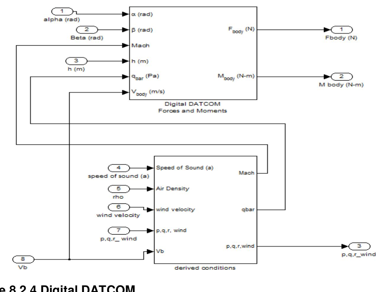Modelling and Simulation of a UH-UAV dynamics 38 School of Engineering and Technology *BEng Final Year Project Report Figure 8.2.3 earth axis The forces and moments are calculated by the Digital DATCOM in the aerodynamic platform. 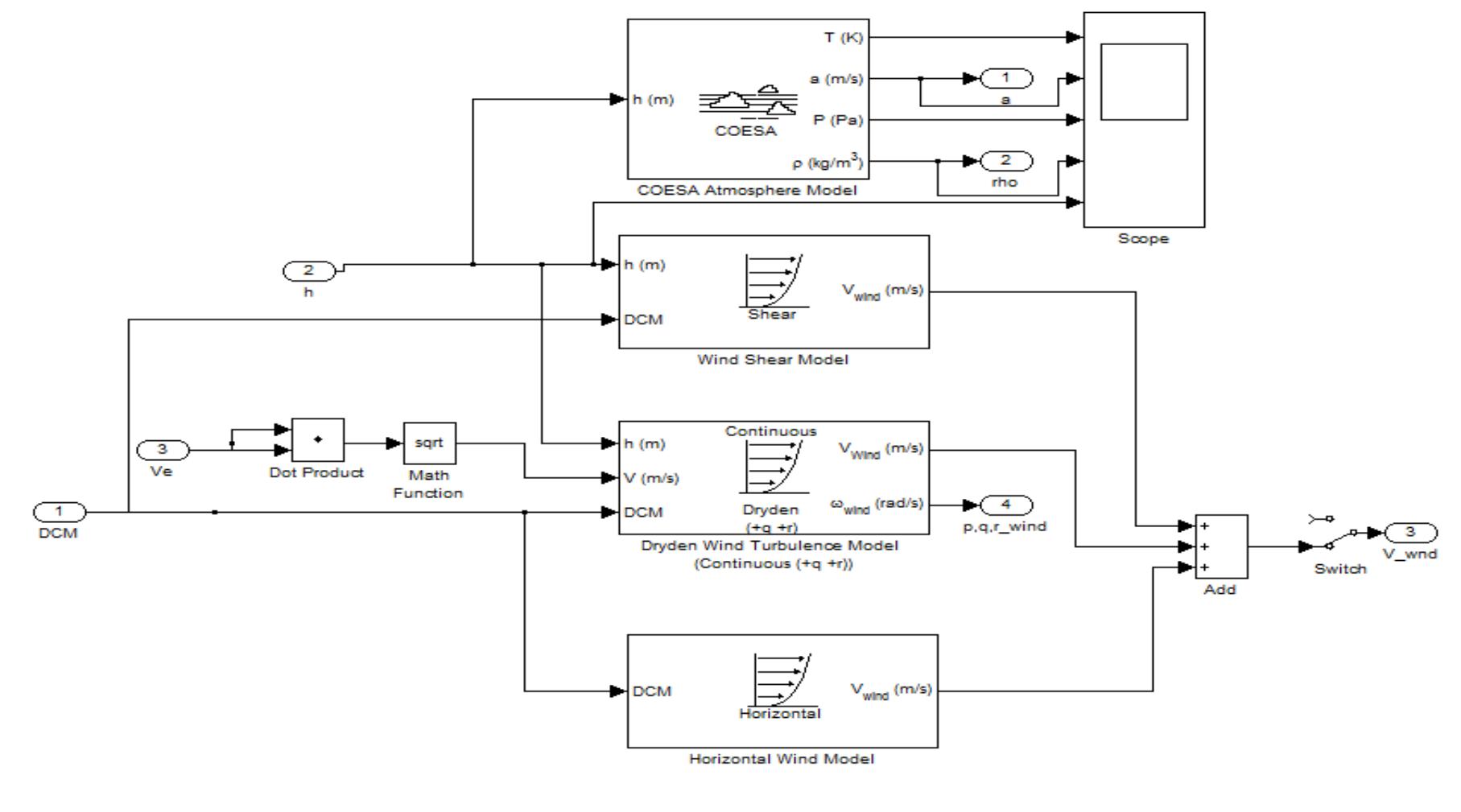Figure 8.2.4 Digital DATCOM The effects atmospheric disturbances such wind Shear, turbulence and crosswinds are computed in the turbulence platform. The COESA atmosphere model uses the geopotential height to determine the absolute temperature, density, pressure and speed of sound at a specific altitude. 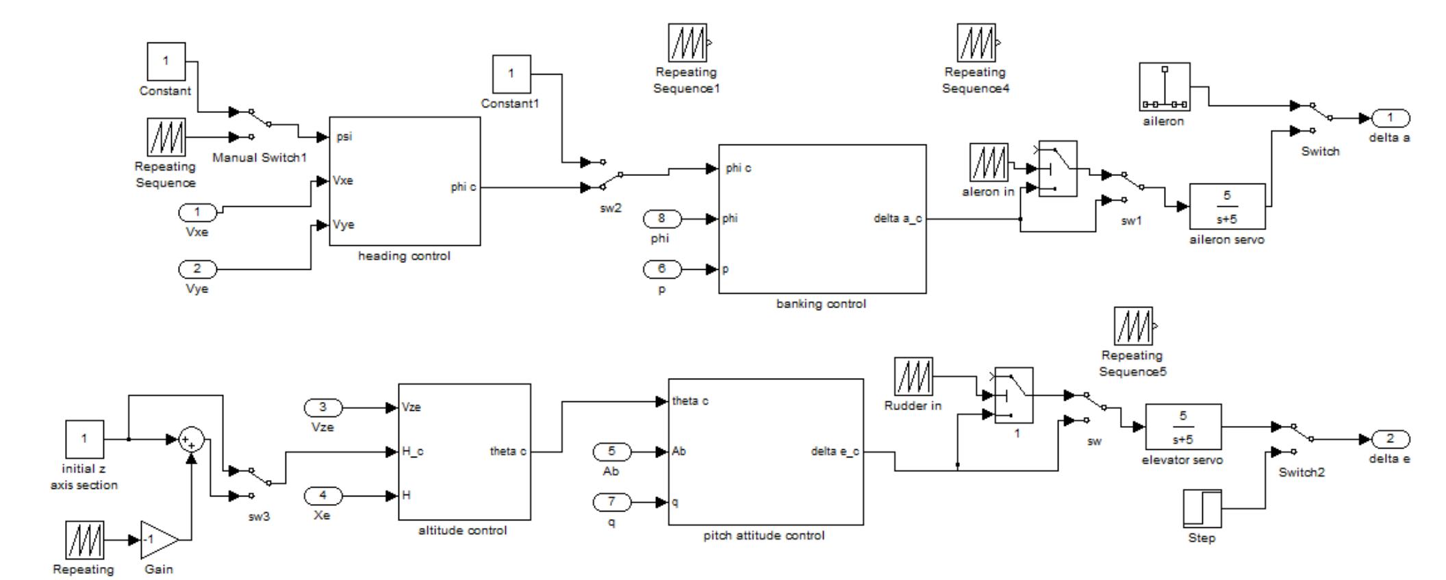Figure 8.2.5 Atmospheric disturbance Modelling and Simulation of a UH-UAV dynamics 39 School of Engineering and Technology *BEng Final Year Project Report Autopilot and flight Augmentation platform The mission can be simulated by entering the control sequences in the UAV autopilot. There is also a feedback loop in each subsystem. This control subsystem can be used for flight augmentation. 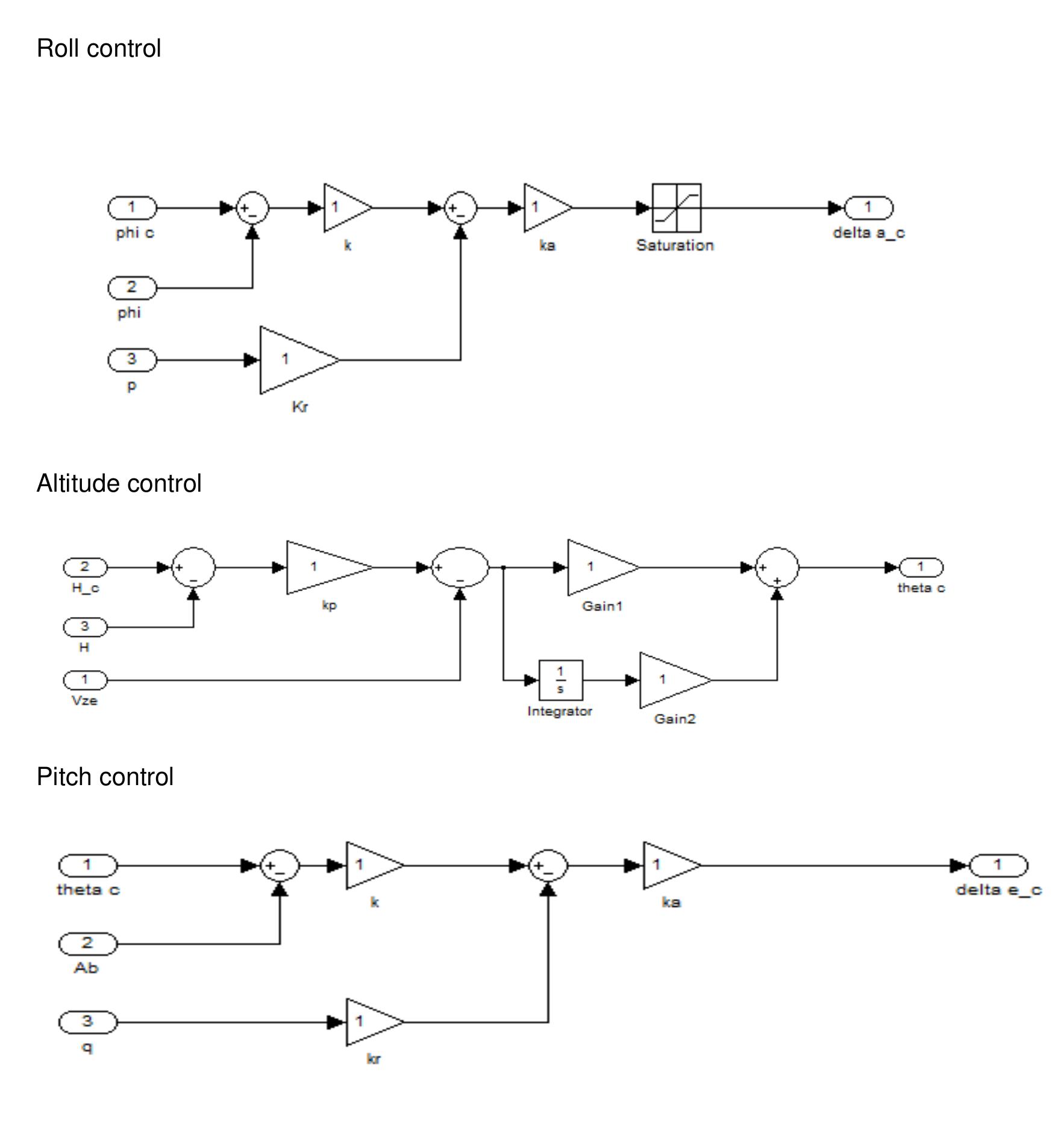Figure 8.2.6 autopilot platform Modelling and Simulation of a UH-UAV dynamics 40 School of Engineering and Technology *BEng Final Year Project Report The UAV flight control subsystems. The gains will be tuned based on the design requirements. 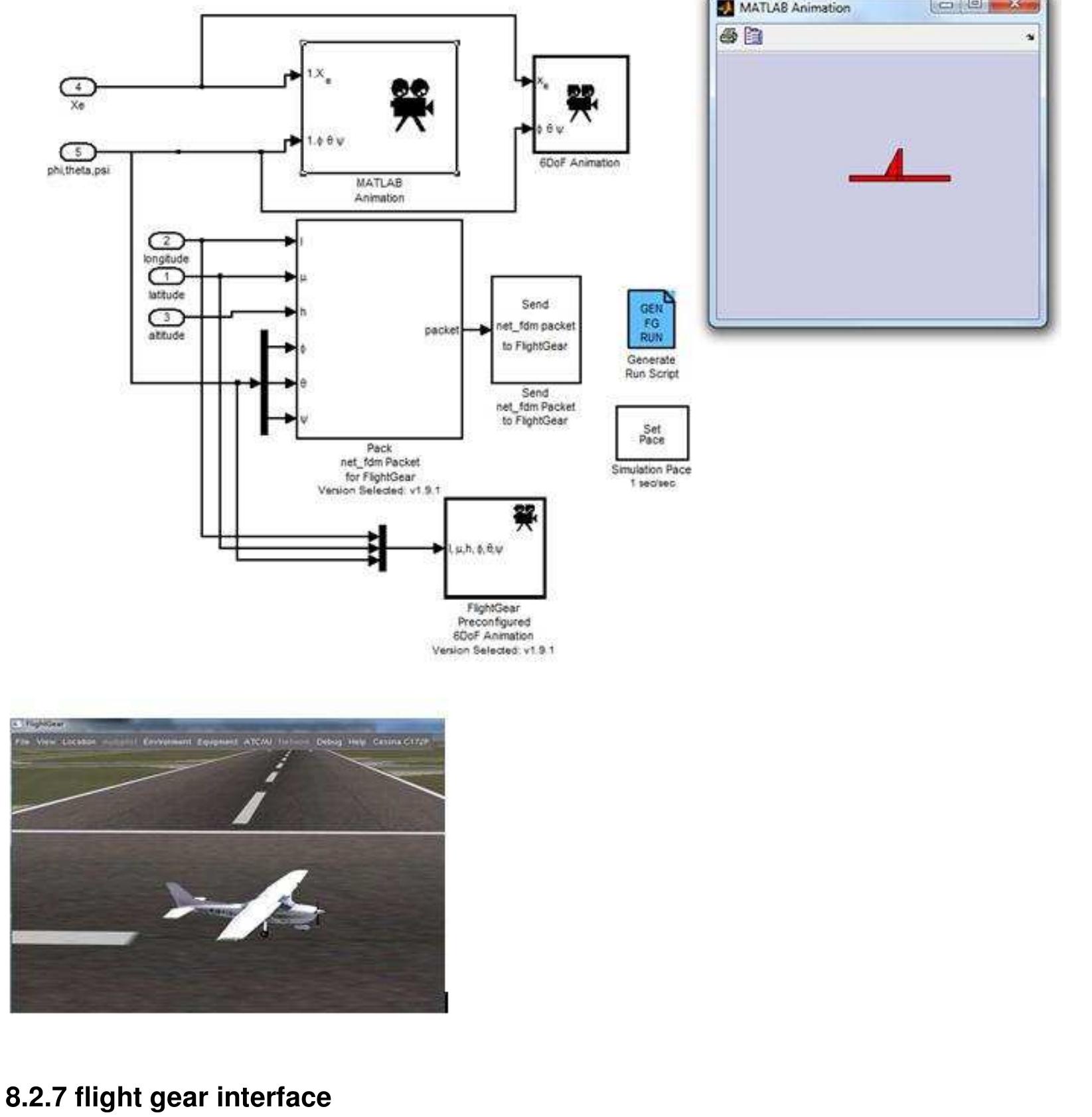Heading control Roll control Altitude control Pitch control Modelling and Simulation of a UH-UAV dynamics 41 School of Engineering and Technology *BEng Final Year Project Report Visual platform The visual platform has interface with flight gear and Matlab based animation. 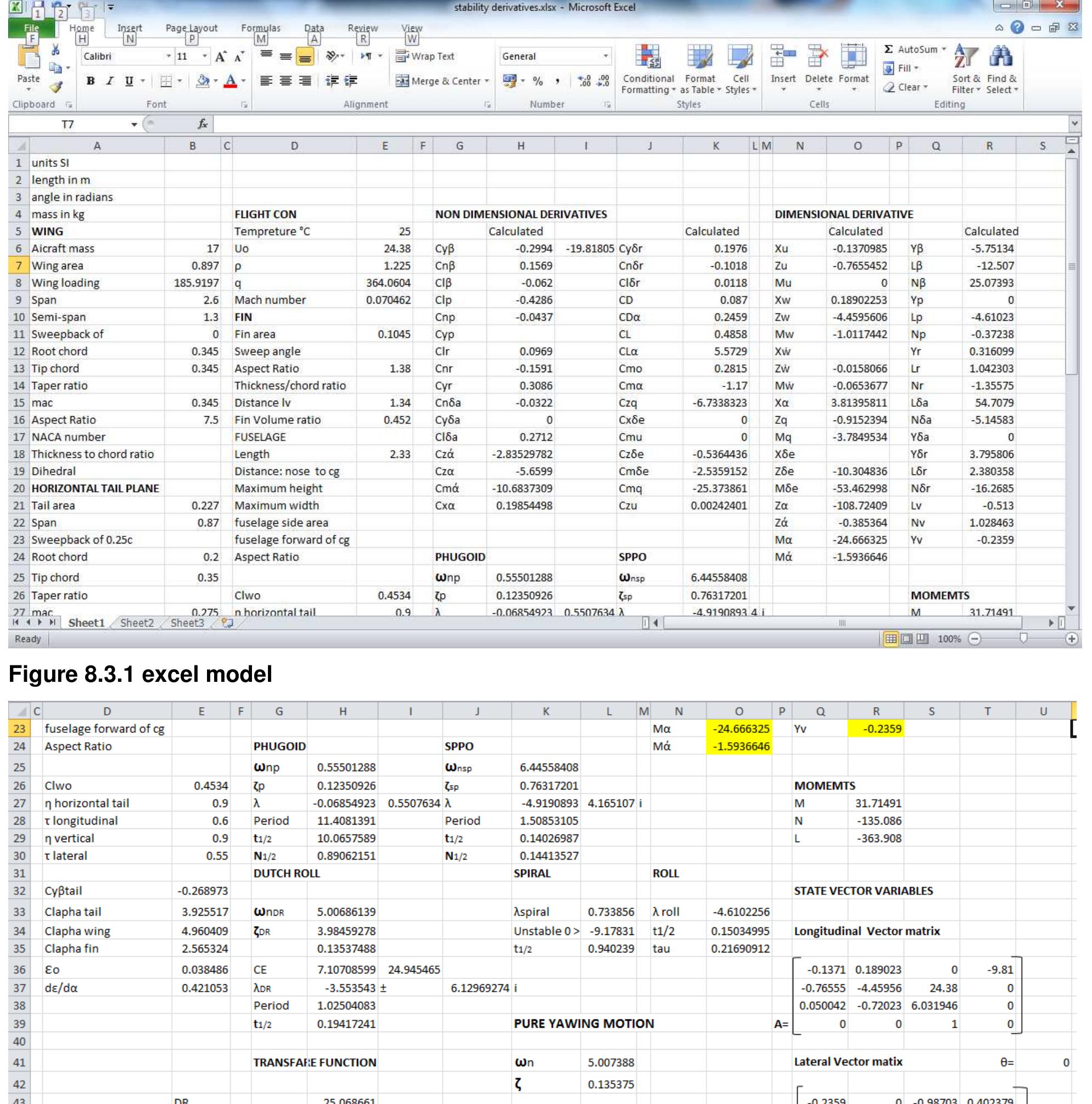Figure 8.2.7 flight gear interface 8.3 The excel model The excel model has a section for inputting geometry parameters and flight conditions. The data for MAK 2 UH UAV was used. 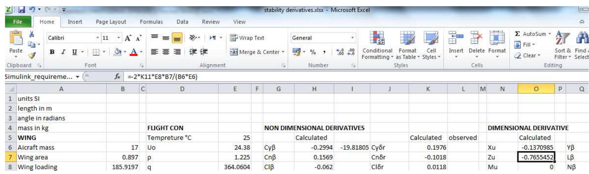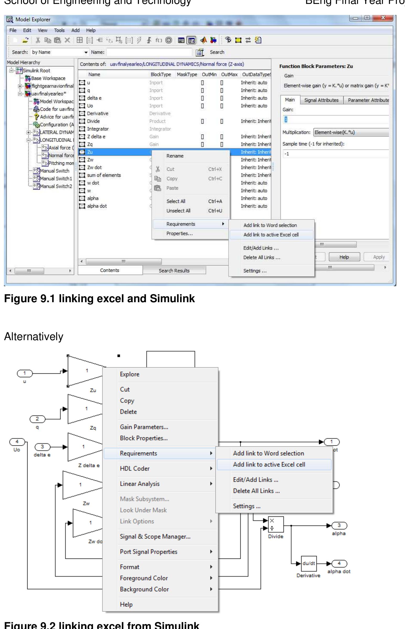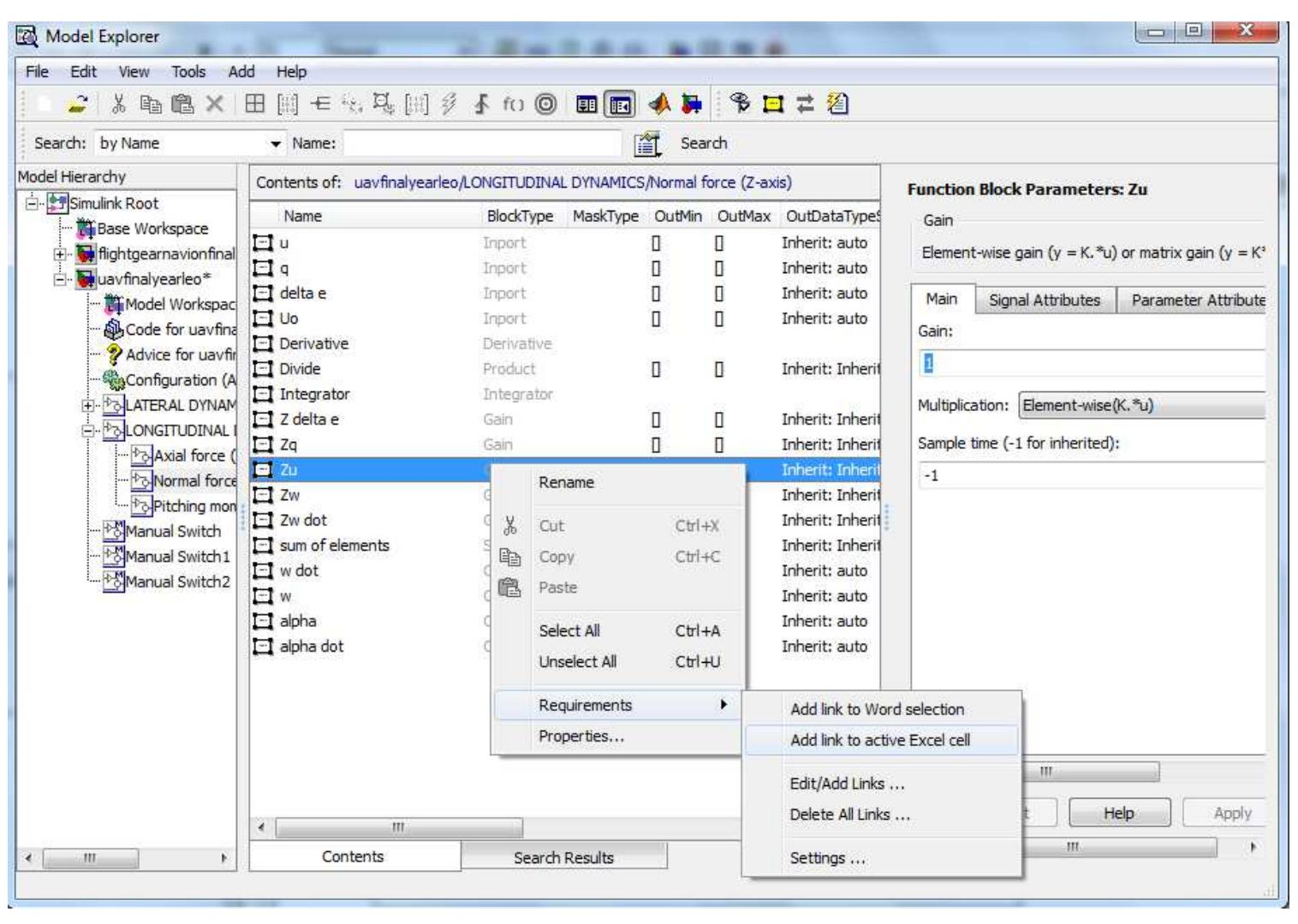Modelling and Simulation of a UH-UAV dynamics 42 School of Engineering and Technology *BEng Final Year Project Report Figure 8.3.1 excel model Figure 8.3.2 excel model 9 Linking Simulink model1 with excel model. 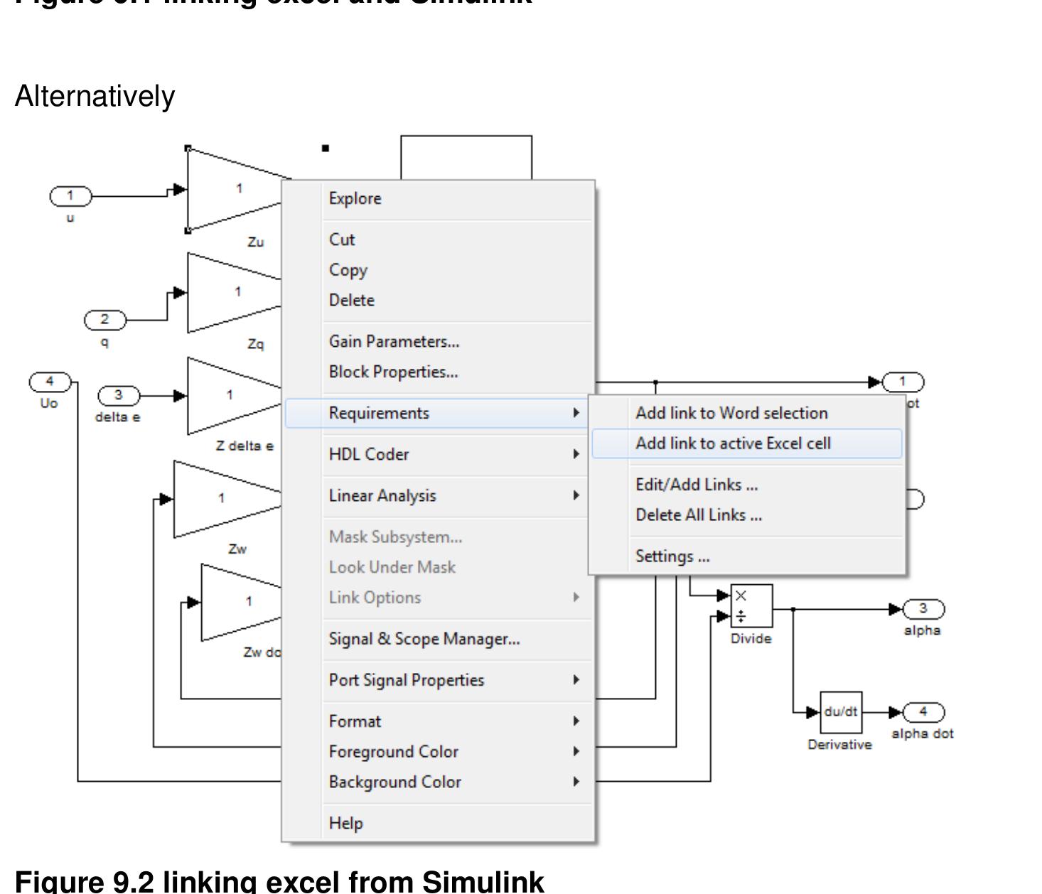Excel model must be open and click the cell to be linked. For instants Zu, then back to Simulink Modelling and Simulation of a UH-UAV dynamics 43 School of Engineering and Technology *BEng Final Year Project Report Figure 9.1 linking excel and Simulink Alternatively Figure 9.2 linking excel from Simulink Excel model actively linked to Simulink. This allows for all flight phases and flight speeds to be simulated. Modelling and Simulation of a UH-UAV dynamics 44 School of Engineering and Technology *BEng Final Year Project Report Figure 9.3 excel Simulink link Summary The MAK 2 UH UAV geometry data was used for the simulations. The static and dynamic stability was defined and further analysed. The derivatives were estimated based on the USF DATCOM method. Recommendations for an optimum UAV geometry configuration were outlined. The derivatives and their effects on stability was analysed in further detail. Two Simulink models were developed. Model 1 further linked to excel and interfaced with flight-gear. This enabled all flight phases to be simulated with automatic updates without recalculating any derivatives. Model Simulink 2 was developed to provide both stability and mission profile simulation. It uses Digital DATCOM to calculate derivatives. Excel model was used to validate the Simulink models by comparing the estimated dynamic characteristics with the observed characteristics. The models can be used to simulate any dynamics of any convectional UAV for any flight conditions. The response to control surface inputs and atmospheric disturbances were determined. The simulations shows that the MAK2 UH UAV has positive longitudinal dynamic stability for the given flight conditions. The MAK2 UAV has a heavily damped SPPO mode and a lightly damped phugoid. MAK2 UH UAV reaches equilibrium position in approximately 84 seconds after a step elevator disturbance. The MAK2 UH UAV has positive lateral stability in roll and yaw disturbances for the given flight conditions. The observed roll time constant was much greater than the estimated roll time constant. Therefore the MAK2 roll rate is less responsive than estimated. The estimation method showed that MAK2 UH UAV is unstable in spiral mode. The research can be used by the UH UAV final year team and UH UAV society to develop an advanced UAV capable of different missions. The stability and augmentation study can be used to design a very stable UH UAV that can also be easily controlled. The simulations can be used for UAV design optimisation, flight testing, and mission simulations. The model is currently interfaced with flight gear. However for further work it can be interfaced with X-Plane which is a more accurate flight simulation that offers flight statistical data for further analyses. 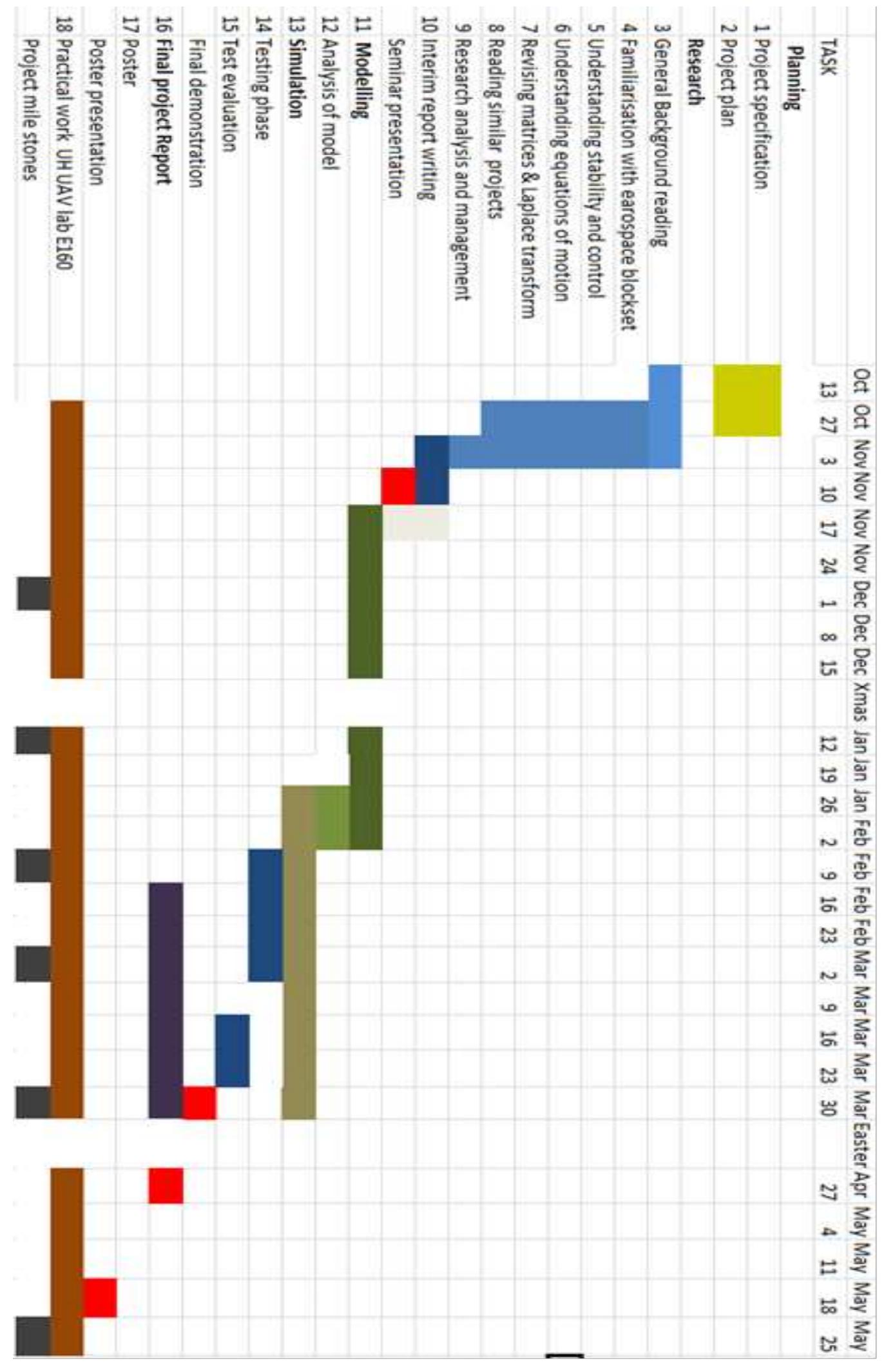Modelling and Simulation of a UH-UAV dynamics 45 School of Engineering and Technology *BEng Final Year Project Report Encountered problems The project was run according to the time plan and it was completed on time. The main problem was getting the data from the other UAV team members. Hence an alternative was to use data from MAK2 an existing UH UAV. The University did not deliver the ordered materials for the actual UAV to be built. However the stability work carried out will be a great contribution to the UH-UAV team. I also contributed by coming up with creative solutions such as using jigs when hotwiring. This resulted in the ailerons being completed in little time. Time plan Modelling and Simulation of a UH-UAV dynamics 46 School of Engineering and Technology *BEng Final Year Project Report References 1. Dictionary of Military and Associated Terms. US Department of Defence 2005 [viewed January 2011], available from: http://www.thefreedictionary.com/Unmanned+Aerial+Vehicle 2. Brief History of UAVs (c) January 2003 LIST lab, University of Florida [Viewed 22 December 2010] available from: http://www.list.ufl.edu/uav/UAVHstry.htm 3. Airborne Autonomous system [Viewed 4 December 2010], available from: http://www.unmannedaircraft.org/page/page/1357249.htm 4. Defence industry daily. An Enhanced Predator for the Army. Gray Eagle © 05 October 2010 [Viewed 22 October 2010] available from: http://www.defenseindustrydaily.com/warrior-ermp-an-enhanced-predator-for-the- army-03056/ 5. BAE SYSTEMS Controls Develops Autopilot for Unmanned Aerial Vehicle Using MathWorks Tools. Feng Liang © 2003 [Viewed 20 October 2010] available from: http://www.mathworks.com/rapid- prototyping/userstories.html?file=45510&title=BAE%20SYSTEMS%20Controls%20D evelops%20Autopilot%20for%20Unmanned%20Aerial%20Vehicle%20Using%20Mat hWorks%20Tools 6. Charles E. Dole, James E. Lewis Flight Theory and Aerodynamics, 2nd edition John Wiley and Sons, 2000, 237 7. Robert C. Nelson Flight stability and Automatic control, 2nd edition McGraw-Hill: Tom Casson,1998, 39 8. Charles E. Dole, James E. Lewis Flight Theory and Aerodynamics, 2nd edition, john Wiley and Sons, 2000, 238 9. Charles E. Dole, James E. Lewis Flight Theory and Aerodynamics, 2nd edition, John Wiley and Sons, 2000, 238 10. Charles E. Dole, James E. Lewis Flight Theory and Aerodynamics, 2nd edition, John Wiley and Sons, 2000,238 11. John Hodgkinson, Aircraft Handling qualities, Blackwell Sciences,1999, 21 12. John Hodgkinson, Aircraft Handling qualities, Blackwell Science,1999, 24 13. Charles E. Dole, James E. Lewis Flight Theory and Aerodynamics, 2nd edition, John Wiley and Sons, 2000, 245 14. Charles E. Dole, James E. Lewis Flight Theory and Aerodynamics, 2nd edition, John Wiley and Sons,2000,245 15. Charles E. Dole, James E. Lewis Flight Theory and Aerodynamics, 2nd edition, John Wiley and Sons, 2000, 247 16. Robert C. Nelson Flight stability and Automatic control, 2nd edition McGraw-Hill: Tom Casson, 1989, 50 Modelling and Simulation of a UH-UAV dynamics 47 School of Engineering and Technology *BEng Final Year Project Report 17. Robert C. Nelson Flight stability and Automatic control, 2nd edition McGraw-Hill: Tom Casson, 1989, 50 18. Charles E. Dole, James E. Lewis Flight Theory and Aerodynamics , 2nd edition, John Wiley and Sons, 2000, 248 19. Robert C. Nelson Flight stability and Automatic control, 2nd edition McGraw-Hill:Tom Casson 1989, 50 20. Charles E. Dole, James E. Lewis Flight Theory and Aerodynamics, 2nd edition, John Wiley and Sons, 2000, 248 21. Robert C. Nelson Flight stability and Automatic control, 2nd edition McGraw-Hill: Tom Casson, 1988, 50 22. Charles E. Dole, James E. Lewis Flight Theory and Aerodynamics, 2nd edition, John Wiley and Sons, 2000, 249 23. Robert C. Nelson Flight stability and Automatic control, 2nd edition McGraw-Hill: Tom Casson, 1998, 63 24. Robert C. Nelson Flight stability and Automatic control, 2nd edition McGraw-Hill: Tom Casion, 1998, 65 25. Robert C. Nelson Flight stability and Automatic control, 2nd edition McGraw-Hill: Tom Casson,1998, 67 26. Charles E. Dole, James E. Lewis Flight Theory and Aerodynamics, 2nd edition John Wiley and Sons, 2000, 259 27. Charles E. Dole, James E. Lewis Flight Theory and Aerodynamics, 2nd edition John Wiley and Sons, 2000 , 264 28. Robert C.Nelson Flight stability and Automatic control, 2nd edition McGraw-Hill: Tom Casson 1998, 65 29. Robert C. Nelson Flight stability and Automatic control, 2nd edition, McGraw-Hill: Tom Casson,1998,81 30. Robert C. Nelson Flight stability and Automatic control, 2nd edition, McGraw-Hill: Tom Casson, 1998, 81 31. Charles E. Dole, James E. Lewis Flight Theory and Aerodynamics, 2nd edition, John Wiley and Sons, 2000, 274 32. Charles E. Dole, James E. Lewis Flight Theory and Aerodynamics , 2nd edition, John Wiley and Sons, 2000, 274 33. Robert C. Nelson Flight stability and Automatic control, 2nd edition, McGraw-Hill:Tom Casson,1998,100 34. Michael. V. Cook Flight dynamics principal, 2nd edition, Elsevier Ltd, 2007, 71 35. Robert C. Nelson Flight stability and Automatic control, 2nd edition, McGraw-Hill: Tom Casson,1998,104 36. Aerospace systems dynamics and control Meng notes, University of Hertfordshire, studynet, 2011 37. Level M flight Mechanics notes , Hertfordshire University, studynet , 2011 Modelling and Simulation of a UH-UAV dynamics 48 School of Engineering and Technology *BEng Final Year Project Report 38. Michael. V. Cook Flight dynamics principal, 2nd edition, Elsevier Ltd, 2007, 381 39. Michael. V. Cook Flight dynamics principal, 2nd edition, Elsevier Ltd, 2007, 381 40. Aerospace systems,dynamics and control MEng notes, Hertfordshire University, studynet, 2011 41. Aerospace systems dynamics and control MEng notes, Hertfordshire University studynet, 2011 42. Aerospace systems dynamics and control MEng notes, Hertfordshire University studynet, 2011 43. Aerospace systems dynamics and control MEng notes, Hertfordshire University , studynet, 2011 44. Michael. V. Cook Flight dynamics principal, 2nd edition, Elsevier Ltd, 2007, 384 45. Michael. V. Cook Flight dynamics principal, 2nd edition, Elsevier Ltd, 2007, 384 46. Introduction to aircraft stability and control 2 ASE4 notes, University of Hertfordshire studynet, 2011 47. Introduction to aircraft stability and control 2 ASE4 notes, University of Hertfordhsire studynet, 2011 48. Robert C. Nelson Flight stability and Automatic control, 1st edition, McGraw-Hill, 1989,159 49. Robert C. Nelson Flight stability and Automatic control,1st edition, McGraw-Hill, 1989,162 50. Robert C. Nelson Flight stability and Automatic control, 1st edition, McGraw-Hill, 1989,162 51. Robert C. Nelson Flight stability and Automatic control, 1st edition, McGraw-Hill, 1989,181 52. Introduction to aircraft stability and control 2 ASE4 notes, University of Hertfordshire studynet, 2011 53. Introduction to aircraft stability and control 2 ASE4 notes, University of Hertforshire studynet,2011 54. Robert C. Nelson Flight stability and Automatic control, 1st edition, McGraw-Hill, 1989,198 55. Robert C. Nelson Flight stability and Automatic control, 1st edition, Mc Graw-Hill, 1989,198 56. Robert C. Nelson Flight stability and Automatic control, 2nd edition, Mc Graw-Hill, 1989,231 Modelling and Simulation of a UH-UAV dynamics 49 School of Engineering and Technology *BEng Final Year Project Report Bibliography 1. Accelerating the space of engineering and science, Aerospace and defence www.mathworks.com/aerospace-defense/ 2. Stevens, B. L., and F. L. Lewis, Aircraft Control and Simulation, John Wiley & Sons, New York, 1992. 3. Smetana, F.O., Computer assisted analysis of aircraft performance stability and control, McGraw-Hill 1984. 4. Babister A.W, Aicraft Dynamics Stability and Response, Pergamon Press, 1980 5. Etkin B, Reid L.D, Dynamics of flight stability and control, 3rd edition, John Wiley and Sons 6. Schmidt L.V, Introduction to aircraft flight dynamics, American Institute of Aeronautics and astronautics, 1998 7. Miller M.P, Accurate method of measuring the moments of Inertia of airplanes, National Advisory Committee for Aeronautics, Washington October 1930. 8. Roskan J, Aiplane Flight Dynamics and Automatic control, 3rd edition, 2001. DARcorporation 9. Turevskiy A, Gage S, Buhr C , Model-Based Design of a New Light-weight Aircraft.The MathWorks, Inc. Natick, MA, 01760 10. Mathworks Matlab help file All the equations used for this project can be obtained from the following books List in order of importance 1. Flight stability and Automatic control, 2nd edition, Mc Graw-Hill by Robert C. Nelson 2. Flight dynamics principal, 2nd edition, Elsevier Ltd, 2007 by Michael .V .Cook 3. 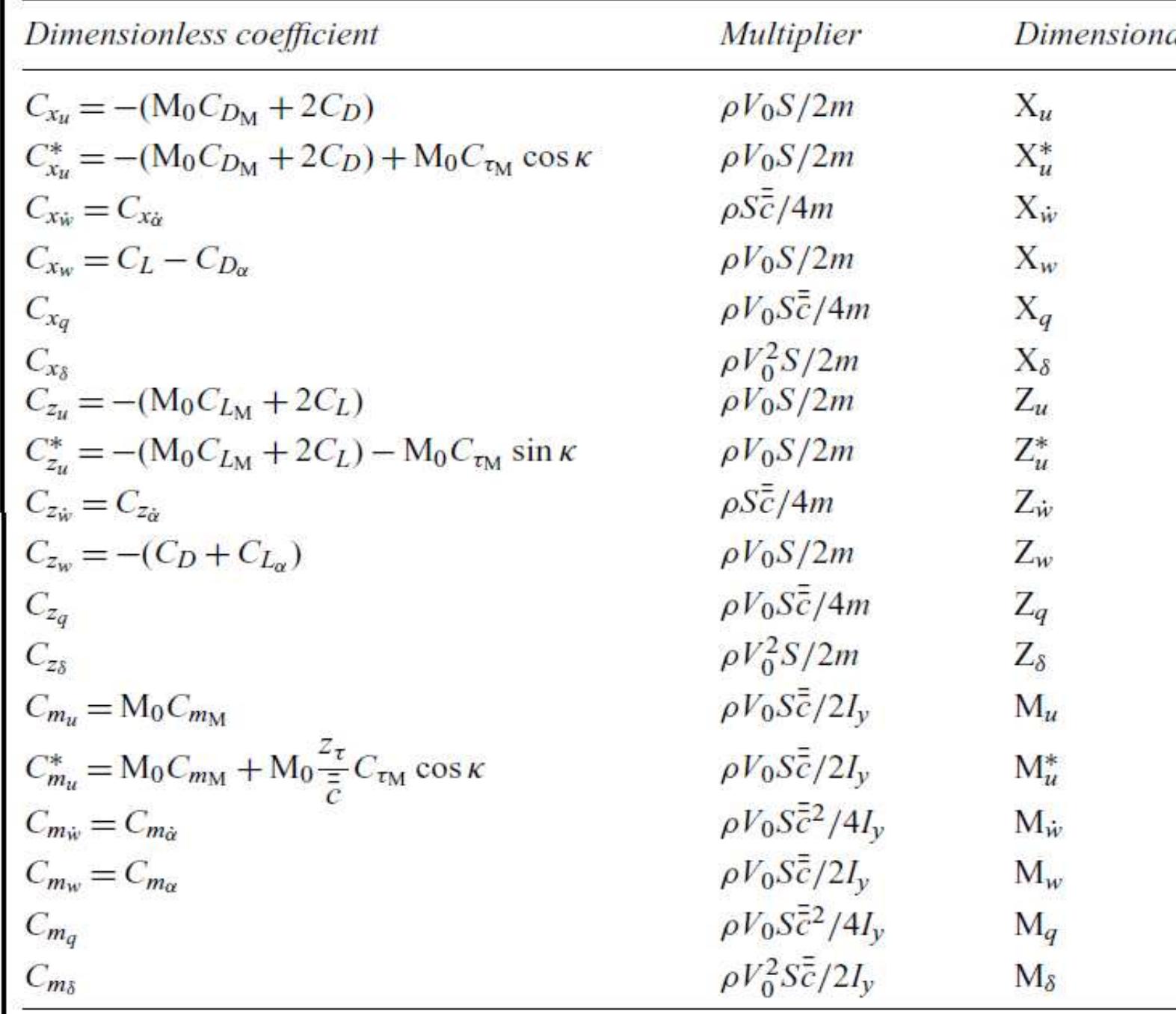Aircraft handling qualities 1st edition, Blackwell Science Ltd , 1999 by John Hodgkinson Modelling and Simulation of a UH-UAV dynamics 50 School of Engineering and Technology *BEng Final Year Project Report APPENDICES APPENDIX A: The longitudinal derivative estimation equations Copy obtained from Michael. V. Cook Flight dynamics principal, 2nd edition, Elsevier Ltd, 2007, 431 Modelling and Simulation of a UH-UAV dynamics 51 School of Engineering and Technology *BEng Final Year Project Report APPENDIX B: Lateral derivative equations Copy obtained from Robert C. Nelson Flight stability and Automatic control, 1st edition, Mc Graw-Hill, 1989,108 Copy obtained from Michael. V. Cook Flight dynamics principal, 2nd edition, Elsevier Ltd, 2007, 432 Modelling and Simulation of a UH-UAV dynamics 52 School of Engineering and Technology *BEng Final Year Project Report APPENDIX C: Eigen vector for gust Modelling and Simulation of a UH-UAV dynamics 53